Sexual Satisfaction Among Slovenian Population

Introduction

Partnership not only satisfies the basic needs of the individual as a social being, but also contributes to health, positive interpersonal relationships, self-confidence, good self-esteem, and general well-being [1,2]. Sexuality is also crucial for good partnership and an important part of the human life cycle [3-5]. Sexual orientation is a predisposing characteristic of a person who is sexually attracted to persons of the same and/or opposite sex. Sexual orientation refers to the gender to which a person is emotionally, physically, sexually, and romantically attracted. It is primarily assessed through personal evaluation and reporting of whether one is attracted to a man or a woman [6,7]. Engaging in sexual relationships with persons of the same or opposite sex most often determines a person’s sexual orientation. Factors that influence whether a person has sex with a person of the same or opposite sex include availability of a partner, moral relationships, social norms, curiosity, need to fulfill the role of a parent, financial motives, etc. [8].
In sexuality it is necessary to separate the masculine and feminine sides. Men are more pragmatic beings, while women are more tactile beings. Therefore, an embrace is of great importance for a woman’s perception of sexuality, as the release of serotonin, dopamine and oxytocin then increases. A woman, who is otherwise a hyperdynamic being and has all her senses constantly activated, usually closes her eyes when kissing. This activates the depilation of the basic system of the visual sense, with which we reach the maximum information capacity of up to 90% [9]. Therefore, the aim of the study was to assess sexual satisfaction in the general Slovenian population using an adapted but modified questionnaire, which was suitable for identifying differences in sexual satisfaction between different variables.

Methods

The study was conducted on female and male participants via online survey. The online survey began in July 2020 and was completed in September 2020. The research was conducted according to the principles of the Declaration of Helsinki. All participants were informed of the aims and anonymity in writing before the study began. Informed consent was given by clicking the “Proceed with questionnaire” button. The National Ethics Committee approved the study design (No. 0120-200/2020/6).
Recruitment was based on the following inclusion conditions:
(a) Age of 18 years and older, and
(b) Personal consent to the questionnaire.
Participants with mental and sexual disorders were also included in the study. All participants were asked for demographic data: gender, age, marital status, education level, sexual orientation, number of children, number of all lifetime sexual partners, number of current sexual partners, number of sexual contacts per month, diagnosed mental and/or gynecological disorders and, for women, the number of archived orgasms during a sexual contact.
A validated questionnaire from Stulhofer, et al. [10] was used with some adaptations that allowed the questionnaire to be completed by both sexes. Linguistic validation of the questionnaire was done by translating it from English to Slovenian and vice versa. The Cronbach’s alpha coefficient showed adequate internal consistency (α=0.963) for all statements. Based on the theoretical content relationship, we grouped certain statements into new cushions/variables:
My mood before sexual intercourse/activity (α=0.936):
• My sexual arousal toward a partner.
• Rate your sexual desire toward a partner
• My sexual response to a partner
• The intensity of my sexual arousal
My mood during intercourse/sexual activity (α=0.854):
• My emotional engagement during sexual activity.
• During sexual activity, I give myself to sexual pleasure
• The intensity of my orgasms
My partner’s mood during intercourse/sexual activity (α=0.936):
• Rate your partner’s sexual activity
• My partner gives in to sexual pleasure
• The way my partner is responsive to my sexual needs
• My partner is sexually creative
• My partner is sexually available
My balance in sexual intercourse/activities (α=0.857):
• Rate the appreciation of the pleasure I give to my partner.
• The variety of my sexual activities
• The frequency of my sexual activities
• The balance between what I give and what I get during sexual activity
• And the autonomic variable:
• My mood after sexual activity.
The modified questionnaire consisted of demographic data and 17 statements. A 5-point Likert scale was used for each statement, ranging from “not at all satisfied” to “extremely satisfied.” Data were analyzed using SPSS 26.0 statistical software. The Kolmogorov-Smirnov test and the Shapiro-Wilk test were applied to determine whether the values had a Gaussian distribution and to choose between parametric and nonparametric statistical tests. The Kolmogorov-Smirnov test and the Shapiro-Wilk test showed a non-normal distribution. Based on this result, a non-parametric statistical analysis was chosen, namely Pearson’s correlation coefficient and χ2 -test. The statistical significance was set at p ≥ 0.05.

Results

A total of 1418 questionnaires were received, of which 474 were fully completed. The realization of the sample was 33.43%. The sample included 405 female (85.4%) and 69 (14.6%) male participants. The basic demographic data are presented in Table 1. Participants were asked about the total number of sexual partners in their lifetime (Table 2). Most had one to two (n=134; 28.3%). Regarding the number of current sexual partners, respondents had one (n=462; 97.5%) or two to three (n=12; 2.5%) sexual partners (Table 2). In addition, the majority of participants had 11 or more (n=98; 20.7%) sexual contacts per month (Table 3). The female representatives were additionally asked about the number of orgasms during sexual intercourse. Most achieved two (n=178; 37.6%), three (n=110; 23.2%), one (n=69; 14.6%), and four or more (n=50; 10.5%) orgasms. Thirty-one (6.5%) participants did not have an orgasm, and 36 (7.6%) responses were missing. Twentysix (5.5%) participants were diagnosed with a mental disorder and 14 (3%) with a gynecological disorder. These individuals were also included in the study as we were interested in finding possible correlations.

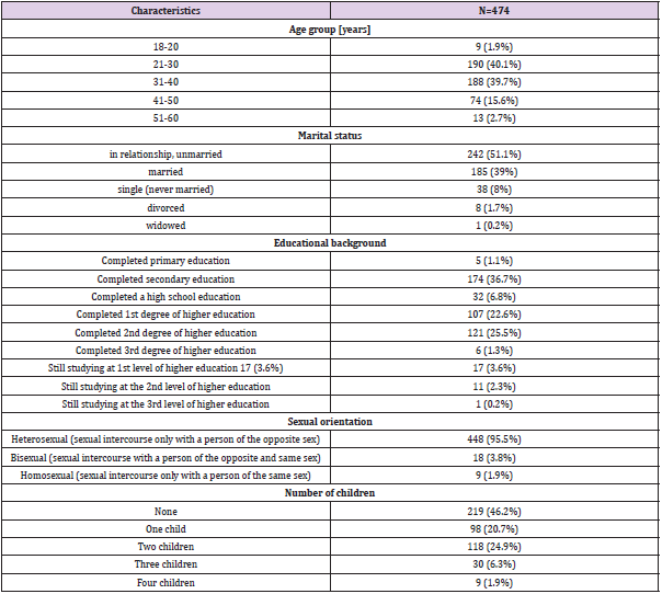
Table 1: Demographic data of the participants.

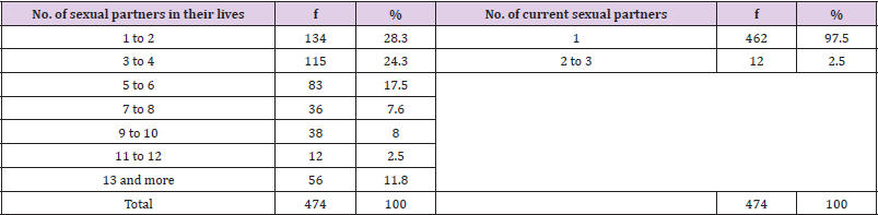
Table 2: Number of sexual partners in their lives and current sexual partners.

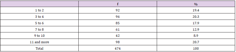
Table 3: Number of sexual intercourses per month.

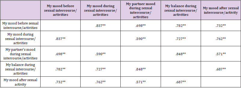
Table 4: Person correlations between the statements.

Note: **. p≤0.01

Based on Pearson correlation coefficient, strong correlations were found between mood before intercourse/activities and mood during intercourse (r=0.837), balance during intercourse/activities (r=0.782), mood after intercourse/activities (r=0.732) and partner’s mood rating during intercourse/activities (r=0.698). There were also correlations between mood during intercourse/activities and mood afterwards (r=0.762), balance during intercourse/activities (r=0.727), and rating of partner’s mood during intercourse/ activities (r=0.590). And between rating partner’s mood during intercourse/activities and balance during intercourse/activities (r=0.848) and mood after intercourse/activities (r=0.571) (Table 4). Female representatives were associated with partner mood and balance within sexual activity (Table 5). Male representatives showed no correlations with any of the cushions. In addition, correlations were found between an age group of 21 to 30 years and mood before, mood during, partner’s mood during, and balance during sexual intercourse/activities (Table 6).

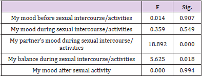
Table 5: Correlation between gender and pillows.

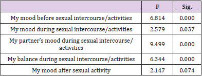
Table 6: Correlation between the age group of 21-30 years and pillows.

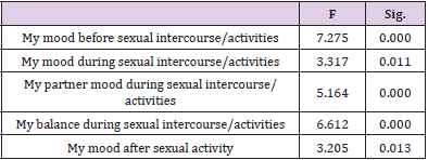
Table 7: Correlation between number of children.

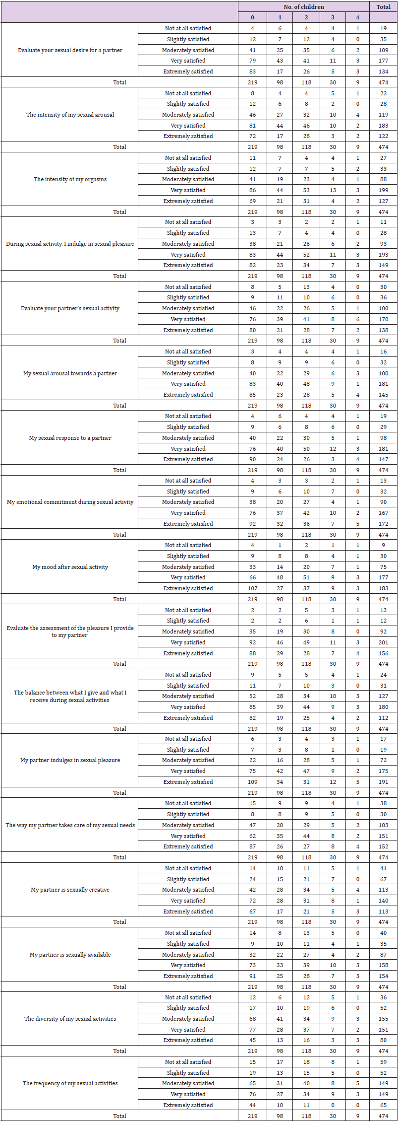
Table 8: Frequency distribution between the number of children and satisfaction-dissatisfaction.

Discussion

Although there are quality of life questionnaires that include questions about sexual satisfaction in the context of chronic disease, there is not much evidence of questionnaires that fully capture sexual satisfaction in the general population. Previous analyses included more women and examined the influence of menopause, body image, psychological distress from chronic disease, discomfort with sexual intercourse, and satisfaction with sexual intercourse. However, as far as we know, there is no questionnaire that includes different variables that could also influence men’s sexual satisfaction. Therefore, the aim of this study was to modify the already established questionnaire to more accurately capture the variables that have an impact on sexual satisfaction, in this case in a general Slovenian population. In our analyses, we included the general population of men and women and even individuals with mental and/or gynecological disorders. The questionnaire was adopted from Stulhofer et al. (2009) and modified to fully capture the sexual satisfaction of men and women from our population.
Based on the achieved reliability of the questions and results, we believe it can be used as a simple tool for clinicians in daily practise to facilitate communication about sexual satisfaction. Examination of correlations between general parameters such as gender, marital status, number of children, sexual intercourse per month, orgasms per activity and dependent variables for sexual satisfaction such as mood before, during and after intercourse and balance within intercourse showed interesting results. Satisfaction correlated well with mood before, during, and after sexual activity and, more importantly, with balance within intercourse. Important here are the questions that measure balance within sexual activity: ‘rating how much pleasure I give my partner’; ‘variety of my sexual activities’; ‘frequency of my sexual activities’; and ‘balance between what I give and what I receive during sexual activities’. This clearly shows that sexual satisfaction depends on the correlation with the activities of the participants and their partners during sexual intercourse. This was even confirmed by the correlations between female representatives and their partner’s mood (F=18.892; p 0.001) and balance during intercourse itself (F=5.625; p=0.994).
In several studies by Basson (2000, 2005, 2015) [11-13], the authors showed that women’s sexual desire is highly dependent on current relationship and partner dynamics, proving that women’s motivation for sexual intercourse does not necessarily arise from sexual desire, but is likely determined by the relationship [14- 17]. In addition, the results of our study proved that previous experience with more sexual partners, higher number of monthly sexual intercourse and orgasms, and younger age were associated with better sexual satisfaction. In addition, participants with more children showed lower sexual satisfaction. Having more children could affect sexual activity and thus sexual satisfaction. Intimacy is an important factor for women with children. The presence of children lowers the level of intimacy as women begin to ignore their sexual arousal because they focus primarily on the children and the family relationship [18,19].
Both were evident in our study, as participants without children were the most satisfied with their sex lives, followed by participants with only one or two children. Satisfaction decreased with the number of children, such that participants with three or four children were the least satisfied with their sex lives. In addition, there were statistically significant correlations between participants who had no children and mood before, during, and after sexual intercourse, partner mood during and after sexual intercourse (both p=0.001), and mood after sexual activity (p=0.013). In addition, Dewitte, et al. [20] showed that the situation of not having children increases sexual activity in women and even decreases the negative effect of sexual desire on sexual activity. Sexual satisfaction was also associated with the age of the participants. Age from 21 to 30 correlated with mood before and during intercourse, mood of partner during intercourse, and balance during intercourse. Increasing age is associated with lower quality of life [21] and therefore could also affect sexual aspects of life, such as number of intercourses per month, number of orgasms, and overall satisfaction.
However, there is a contradictory variable that could affect sexual satisfaction. Namely, in our study, the number of sexual partners also showed a correlation with satisfaction. In this case, we would expect older participants to have better sexual satisfaction than younger ones, but this was not the case. One reason for this is the specificity of the questionnaire we used in our study. The questionnaire specifically addressed sexuality and sexual activity rather than overall quality of life. A middle-aged person may have a higher quality of life than a person aged 21 to 30 because their life priorities lie elsewhere. Here we have not come across the financial influences, career, family and social status. These are all factors that significantly affect the quality of life. On the other hand, life experience in sexuality, as people learn more about their sexual preferences or those of their partner over the course of their lives, could also be an interesting influencing factor on sexual satisfaction. This is suggested by the study of Forbes, et al. [21], who found opposite results when examining sexual quality of life with age.
They observed a positive relationship between age and sexual quality of life. Accordingly, for older participants, the quality – rather than quantity – of sexual encounters was a more important predictor of higher sexual satisfaction. In our study, we did not specifically measure quality per se, but attempted to estimate quality based on pleasure, number of sexual encounters, and orgasms. This could be the reason why younger participants experience better sexual satisfaction than participants in older age groups. The number of sexual encounters became less influential with age [22]. However, in both reports, age was associated with a decrease in sexual aspects of life. Our modified questionnaire was informative enough, showed good reliabilities of variables of significantly above 0.8, and can potentially be used in daily clinical practice.
However, there were limitations in this study. Despite the large sample size, the questionnaire should be validated in further studies to obtain additional information about the reliability of the questions. Also, more comparisons should be made between different parameters such as gender, marital status, and sexual orientation to gain truly meaningful insights into the variables that influence sexual satisfaction. In addition, a larger sample of men should be included in the future, as the results cannot be generalized to the general population due to the predominantly female participants. As this study was designed as a pilot study, we intend to conduct further analysis and gather further insights as we consider the questionnaire to be meaningful enough.

Conclusion

The present study provided the results that previous experience with more sexual partners, higher number of monthly intercourse and orgasms, and younger age were associated with better sexual satisfaction. In addition, participants with more children showed lower sexual satisfaction. In addition, a newly modified questionnaire was used for the first time to assess sexual satisfaction in male and female representatives. The questionnaire was evaluated and can be used in clinical practice to assess the level of satisfaction with sexual life. By measuring sexual satisfaction using mood pillow ratings, the questionnaire is a suitable tool for further evaluation and for a larger sample to obtain additional data on factors that might influence sexual satisfaction.

For More Articles: Biomedical Journal Impact Factor: https://biomedres.us

Review of Temperature Measurement Techniques

Introduction

Phase change phenomenon involves instantaneous variations of the local heat transfer, which is coupled to the unsteady fluid currents overlying the surface. An example is the sessile drop, which is of interest in several fields including coating, combustion, and cooling facilities. Understanding of these mechanisms requires fine spatial and temporal measurements, which is essential for applications associated with design optimization and safety consideration of a process. Such consideration is crucial within the operations of boilers, for instance, where the evolved heat flux is restricted by the boiling crisis. This operational regime is often associated with equipment failure. Within the miniaturized electronics applications such as transistors, high heat fluxes up to 200 W/cm2 can be liberated from such instruments, where a low wall superheat is desired with respect to the cooling fluid. Thus, operating within the correct boiling regime becomes paramount in the thermal management of the operating equipment [1-4]. In addition, some of the proposed models are not well validated due to the limited resolution of the available data, which might bring about a misinterpretation of the phase change phenomenon under study. Such situations can be encountered with respect to models based on point measurements, which cannot resolve fine spatial resolutions associated with phase change phenomenon [5-6]. In the current paper, some of the relevant temperature measurement techniques are provided, which include point measurement techniques and IR thermography. A review of fluorescing materials and their usage within temperature measurement applications are given by the end of the paper.

Point Measurements

A conventional point measurement technique is the thermocouple, which operates on the basis of Seebeck effect. In principle, two dissimilar metals are connected at a junction, which generates a small voltage with respect to a given temperature. Such technique was used to acquire average heat flux measurement over a surface of interest [6]. In parallel to this technique, Truong [7] considered using a heat fluxmeter, so as to evaluate the heat transfer coefficient associated with a heat sink, via Newton’s law of cooling. The drawback of such methods is that its usage is limited to quasi-steady state regime, which cannot be used for complex flow phenomena, due to multidimensionality and the instantaneous local changes of the fluid-wall interaction [6-7]. In case of the heat fluxmeter, significant measurement error can incur, in case the thermal properties of the instrument was not well quantified [7].

Resistive Based Sensors

In the past decades, thermal resistance-based sensors has been the focus of wide of variety of applications. These include thermal actuator, flow rate and temperature measuring devices, and sensors pertaining to gas monitoring within food logistics [8-10]. Several studies focused on developing high compact microheater sensors, with competitive spatial resolution performance. Such advances were permitted with development of microfabrication, which enable one to realize fine features as small as a submicron length. Such sensors can play a crucial role in detailed examination of adverse flow condition, as in phase change application for instance, which can be achieved by its instantaneous measurement at multipoint resolution and its conformity to nonplanar surfaces [11-14]. Among the various works on resistive sensors, is the one done by Guereca [15] in the field of microelectromechanical systems, which was used in boiling application. The instrument used in Guereca [15] study was fabricated via ion beam milling and photolithography, which had a dual function of providing heat to surrounding fluid and for temperature measurement purposes. The latter used to measure the nucleation temperature, based on sudden changes in the observed temperature, with respect to the temperature coefficient of the instrument resistance [15]. Figure 1 depicts the microheater array used by Demiray and Kim [16] within FC-72 pool boiling experiment.

Figure 1: Micro heater array for pool boiling experiment (left), heat transfer distribution under nucleating bubble at micro heater surface (right) [16].

Some of the major challenges with respect to the sensor’s fabrication regard the dimensional scale difference between the patterned lead connection and the deposited sensor metal, which is one of the main causes for electrical disconnection, due to the sensor’s breakage along the lead’s edges. Such issues are further complicated if an adhesion layer exist between the flexible substrate and the pattern leads. In addition, it is crucial to include a thermal insulation within the metal sensor design, which can affect its performance criteria, such as measurement sensitivity and resolution [11-12,17-19]. Also, some studies have indicated deviation of the material properties from bulk metal value for thicknesses close to the mean free path. For instance, Siegel, et al. [20] observed an inverse relation between resistance and temperature for gold thickness of several nm, as opposed to the proportional correlation between resistance and temperature for bulkier gold thicknesses. Inhomogeneity in the deposited sensor can lead to large temperature gradient on the sensor’s surface, which can affect the integrity of the temperature measurement. For instance, Guereca [15] noticed that the acquired temperature measurement was lower for thinner fabricated resistive sensor. Lastly and not least, such temperature measurement requires direct contact with fluid of interest, and it has an element of Joule’s heating. Thus, there is some form of intrusion upon the investigated phenomenon, which might induce some form of error.

Non-Contact Local Temperature Measurement Techniques

A breakthrough in surface temperature measurement has been achieved recently, via infrared (IR) technology, which permitted local heat flux measurements at fine spatial resolution. Such technique proved to be of an essence in proper understanding of heat transfer mechanism, and to further elaborate existing models and correlations.

Infrared Thermography

Several studies utilized Infrared (IR) technique in order to resolve the local wall heat transfer in both pool and flow boiling applications. An example is the study conducted by Scammell and Kim [21], where they examined the effect of vortex shedding upon the local wall heat transfer in flow boiling applications. A schematic of the flow boiling test section is shown in Figure 2. The IR measurements in such studies are based on black coating of the wall surface, adjacent to the working fluid, which acted as temperature markers for the IR camera. The temperature profile across the wall was deduced numerically, in a coupled radiationconduction problem from which the local heat flux profile was resolved [21].

Figure 2: Flow boiling test section setup featuring golden mirrors for simultaneous heat transfer measurements and flow visualization (left image), and cross-sectional view of the flow boiling test section (right image) [21].

Some of the major obstacles associated with IR thermography, pertains to the availability of the IR optical properties, which is required to resolve the temperatures across IR transparent materials, such as silicon and Kapton tape [6,22-24]. Not to mention that IR transparent materials are not easy to machine, such as in the case of CaF2 [25]. In addition, in case there is a sharp temperature gradient, there is a restriction on the minimal number of pixels covering an area, so as to resolve the spatial temperature distribution at a region of interest [22-23]. Jason [23] has also raised an issue pertaining to the integration time with respect to the calibration range, where an error in the order of 10 degrees can incur, in case the measurement was done outside the calibration range.

Time Domain Thermoreflectance

Another non-contact measurement technique is the time domain thermoreflectance (TDTR), which relies on the examining the material reflectance property variation with temperature. A schematic of the TDTR technique is shown in Figure 3. Such approach is applied in order to determine the thermal properties of materials, which is of interest within the development of new materials, including nanomaterials and thin films. In a study by Mehrvand and Putnam [24], the heat transfer coefficient at the thermal boundary layer within a flowing fluid was examined using TDTR technique. One of the advantages of the TDTR techniques is its spatial resolution relative to IR thermography, due to its use of visible light. On the other hand, TDTR requires a complex setup, which involves various optical equipment and probing instrumentations. Therefore, its generally not applicable to the complex geometries that can arise in boiling heat transfer application.

Figure 3: TDTR setup for material thermo conductivity measurement (ww.nist.gov/programs-projects/measurements- and-standards-thermoelectric-materilas).

Fluorescing Measurement Techniques

The following subsections summarizes the measurement techniques that utilizes photoluminescent materials, such as liquid crystals and quantum dot. Such measurement approach relies on the spectral emission variation of such materials temperature, which can give a fine spatial resolution of the surface measurement.

Liquid Crystals

Thermographic techniques based on liquid crystals and fluorophores has been suggested as a temperature indicator. One such an attempt is the work done by Kenning [26], where he examined the wall temperature profile within nucleate boiling application, via a thermochromic liquid crystal. However, such techniques can involve tedious calibration procedures and limitations associated with equipment availability and operating costs [27-30]. Not to mention, the narrow temperature operating range by liquid crystal technique [25].

Quantum Dots

Quantum dots (QDs) are semiconductors whose length scale is in the order of nanometers and thus subject to 3D confinement. QDs have unique optical properties relative to traditional fluorophores in which it can be excited by a wide range of wavelengths. In addition, it emits light over a narrow spectrum at a longer wavelength, which can easily be captured using a long pass filter. Solid-state lamps in the form of LEDs are usually used for QD excitation purposes. As a direct consequence of the QD length scale, the color of the emitted light can be tuned by changing the QD size via temperature and synthesis time control of the fabrication process. Examples of QDs spectrum emission variation is shown in Figure 4. QDs are prepared in a colloidal liquid, and it can easily be transferred to surfaces of interest via spray or spin coating. Such versatile fabrication processes can greatly downsize the expenses, pertaining to facility complexity [31-38]. Other QDs delivery methods include electrostatic coating, UV curable solutions, as well as sol-gel approach [38-42]. According to the airy diffraction theory, the minimum spatial resolution that can be detected by a camera (x) is related to the observed wavelength (λ) by Equation 1. In Equation 1, f is the distance between the lens and object and d is diameter of the aperture. Thus, QD has a spatial resolution advantage over IR thermography, where local heat flux measurements can be acquired at submicron ranges, due to its smaller wavelength emission [43].

xf =1.22λd (1)

Figure 4: QD, (left) emission from dots of increasing size from left to right (Wikipedia.org/wiki/quantum_dot).(right)Spectral characterization of QD.

Another characteristic of QDs is the temperature dependency of their optical properties as shown in Figure 5, which can be exploited for temperature measurement purposes. This can be related to stoke shift behavior of QDs, which is related to the photoluminescence peak shift, as was observed in previous studies [33,37,44-46]. The temperature variation alters the QD optical properties due to thermal expansion of the QD structural lattice [30,36]. Two trends are evident. The intensity of the emitted light tends to decrease with temperature and the peak in the emitted spectrum tends to shift to longer wavelengths. The changes in the intensity and peak wavelength spectra are not necessarily proportional with temperature. The emitted light intensity changes with temperature tend to be quadratic, which makes it less precise than spectral measurement over large temperature ranges [37,45].

Figure 5: Quantum dot optical property variation with temperature [44].

Relative Intensity
1.00
0.80
0.60
0.40
0.20
0.00
360 410 460 510 560 610 660 710 760
Wavelength (nm)
Several studies have used QDs to measure temperature. Al Hashimi and Kim [47] investigated the local heat flux distribution arising from the vaporization of an ethanol drop, where QDs dispersed within a gelatin film were used to acquire surface temperature variation underlying the ethanol drop. The experimental setup for the ethanol drops temperature measurement is given in Figure 6. Matsuda, et al. [31] used ZnSAgInS 2 QDs for surface temperature measurement due to their low toxicity and high temperature sensitivity. Jorge, et al. [33] achieved independency from the excitation source intensity by using multiple QDs with different emission spectra and looking at the intensity ratio. Sakaue, et al. [34] developed a QD temperature sensor for cryogenic application. Li, et al. [44] examined the temperature profile of a micro-heater by calibrating the spectral shift of QDs with temperature. They emphasized the importance of QDs particle concentration on a surface so as to achieve a certain temperature precision as a result of particle size variation [44].

Figure 6: Ethanol drop experimental, (left) test setup, (right)QD-gelatin film.

The average temperature precision was enhanced at a higher number of QD particles, according to Li et al. [44]. Wang et al. [39] developed a miniaturized temperature sensor in the form of a reflective fiber for high temperature applications. In a similar line of work to Wang et al. [39], Bueno et al. [37] developed a photonic planar waveguide temperature sensor using nanocomposites of CdTe and CdSe, which were embedded in PMMA. QDs-PMMA nanocomposites have a peak spectral emission at a shorter wavelength than colloidal solutions of QDs, due to the particles agglomeration and waveguide effects introduced by PMMA matrix. In addition, PMMA tends to be hydrophobic, which minimizes the effect of humidity upon temperature measurement [37]. One of the issues pertaining to QDs can be related to the photobleaching degradation of the emission, which is associated with the breakdown of QDs as a result of continuous light excitation. Other issues pertain to the temperature calibration, which is sensitive to the observed noise in the QD emission readings. Such issues can be remediated by utilizing a high quantum yield of QDs, or photoluminescence emission, and by utilizing CCD cameras instead of CMOS cameras for higher signal to noise ratio [33-34,48-49]. Yu, et al. [45] reported an initial blue shift of the QDs peak spectral emission to shorter wavelengths during the first heating and cooling cycles. Such behavior was resolved by exposing the QDs to several thermal cycles, which resulted in a reproducible spectral peak emission with respect to temperature. Other issues pertain to photooxidation, which can cause an irreversible blue shift due to interaction with surrounding gases [48]. Also, the concentration variation of QDs on a particular area can bring about an uneven intensity distribution, since it’s difficult to control the uniformity of QDs over a surface [38,44].

Temperature Sensitive Paint

Another fluorescing material that works under the same principle as the quantum dots is the temperature sensitive paint (TSP), which comprises of a light emitting luminophores and a binder. As shown in Figure 7, the luminophores gets excited to a higher energy state upon absorption of photons from a short wavelength light source. Afterwards, the excited luminophores undergoes a decay to a lower energy state, where it emits light at a longer wavelength. This process is called photoluminescence. Two conversion processes compete with the photoluminescence of the TSP, which causes the luminophores to decay closer to its ground state: first, the external conversion of the luminophores energy, which is associated with its emitted light quenching via molecular interaction. Such process is relevant within pressure sensitive paint applications, where various oxygen concentrations are associated with different light emission intensity from the luminophores. The second type of the luminophores conversion processes is the internal conversion, which is associated with the energy state variation of luminophore with temperature. Such process is called thermal quenching [25]. The material selection for the luminophores and the binder governs the optical characteristics of the yielded TSP. For instance, the temperature dependency of the luminophore’s light emission varies from one material to another. In addition, the operation of the paint as a temperature sensitive or pressure sensitive paint depends on the binder permeability to oxygen [50]. Recent interest in TSP has emerged in several applications, as a local temperature measurement mean.

Figure 7: Jablonsky energy-level diagram [25].

One of those attempts is the work by Al Hashimi, et al. [51], where Ruthenium based TSP was used to measure the local heat flux distribution within both pool boiling and flow boiling application. Figures 8 & 9 illustrate the test section set up within the pool boiling experiment, where the local heat flux distribution was acquired using the inverse heat conduction problem. The temperature measurement across the adhesive layer was used as boundary conductions for the heat conduction problem, where the heat evolved to the boiling fluid was evaluated as the difference between the heat generated at the NiCr heater and the heat lost to the Sapphire substrate. In Shibuya, et al. [52] study, local temperature variation was captured in form of TSP intensity changes, as a consequence of a passing bubble. Several studies utilized TSP optical properties for surface temperature measurement within wind tunnel facilities some of which were involved in hypersonic flow conditions.

Figure 8: Schematic of the test section.

Figure 9: Depiction of the germanium dot and NiCr heater.

Among the various wind tunnel experiments are the work by Kurits [53], Bhandari [54], Lee, et al. [50], Schramm, et al. [55], Huang [56], Yang, et al. [57] and Ozawa et al. [58], where the local temperature distributions were deduced from surface of interest, based on the observed TSP emission. In more recent study by Liu and Risius [59], TSP is used for thermal imaging purposes within high-enthalpy shock tunnel application. Within Liu and Risius study, a reliable heat flux sensor was used in conjunction with an in-situ calibration technique, so as to determine the thermal penetration within the TSP layer, via an analytical inverse solution [59]. Long [60] utilized multiple luminophores one of which is temperature insensitive, so as to account for the intensity variation within the excitation light source. In a study by Huang, et al. [61] examined the temperature profile within a microchannel flow application, via the optical properties of the TSP. Simultaneous flow visualization and thermal profiling was achieved by Matsuda, et al. [62] for a multiphase flow phenomenon, within microchannel applications. In Matsuda study, TSP was used to survey the temperature profile at various flow boiling conditions, where the acquired Nusselt number was in good agreement with the Sieder- Tate equation [62]. Other work by Ishii and Fumoto [63] utilized TSP in order to acquire temperature distribution at the evaporator wall of a pulsating heat pipe. From the temperature data analysis, a correlation was acquired between the temperature distribution and the observed oscillatory flow phenomenon within the pipe. In addition, a temperature accuracy of 0.263°C was reported within Ishii and Fumoto study [63].

Recent interest in luminophores utilization was found in other applications, such as its usage as PSP. Examples are the studies carried out by Jiao, et al. [64,66,67]. In Jiao, et al. [64] study, a twodimensional correction factor was adopted in the data analysis, so as to resolve the temperature sensitivity of the PSP. Such result was validated against CFD data. In another study by Noda, et al. [66], PSP was used to resolve the transient pressure field on a NACA 0012 airfoil. Other applications for PSP include jet impingement, such as the study carried out by Li, et al. [67], where it was used to examine the pressure field characteristics near the impingement point, such as the nozzle-plate distance, impingement angle, and pressure ratio. The luminophores suffer from similar shortcomings as the quantum dots. For instance, paint thickness inhomogeneities over the surface as well as non-uniform excitation light illumination are among several factors attributed to the observed noise within optical measurements. Background noise and particulates can also interfere with the optical properties of the TSP, which can bring about a shift in the observed intensities. Photobleaching effect tends to be more severe in the case of TSP [68]. In a recent study by Liu et al [69], the temperature dependency of the thermal diffusivity parameter was addressed within the TSP heat flux measurement, which can arise within hypersonic wind tunnel applications. A correction factor was developed within Liu et al study, which was validated against simulation data [69]. Other issues pertaining to the error arising from the TSP apparent temperature relative to the actual wall temperature, as was suggested in a study by Liu, et al. [70]. Such discrepancy becomes more prominent as the thickness of the TSP layer increases, relative to adjacent layers [70].

Conclusion

In the current review paper, various temperature measurement techniques were examined, along with their applications in various research works. Conventional temperature measurement techniques include thermocouple and microheater arrays, where thermocouples can misrepresent the local interaction at the measurement surface, due to its spatial limitation by its average measurement approach. On the other hand, microheaters are complex to fabricate and are difficult to install on non-flat geometries, such as tubes. In the past decade, IR thermography was adaptedas a measurement technique, which can monitor the temperature distribution at a micron resolution. Therefore, an enhanced measurement fidelity can be achieved with respect to the investigated phenomenon. Some of the drawbacks of the IR technique is its compatibility with the measurement surface, which can be opaque to the IR wavelength or are generally expensive to acquire. Novel temperature measurement approaches involve fluorescing materials, which act as a potential alternative to IR thermography. Such materials include QDs and TSP, which operate within the visible wavelength. Hence, a broader range of materials can be used as a substrate for the experiment, where an affordable monochromic camera can be used for local temperature measurement purposes in various applications, such as pool boiling.

Conflict of Interest

No conflict of interest with any institution/organization.

For More Articles: Biomedical Journal Impact Factor: https://biomedres.us

Introduction

The COVID-19 pandemic has created an unprecedented need for diagnostic testing. In early 2020, diagnostic manufacturers were still struggling to raise the capacity of the new COVID-19 test to a reasonable level, but due to limited supply and high demand, prices became a challenge to low- and medium-income countries [1]. COVID-19 screening tests are essential in tracking where countries are in terms of COVID-19 and how far they need to act to combat /and manage it. There are two types of tests currently being conducted, namely the COVID-19 Polymerase Chain Reaction (PCR) and Rapid Antigen Tests. The PCR tests whether a person has the virus, whereas the Rapid Antigen tests whether a person has developed antibodies against the virus, assuming they have previously contracted the virus and whether their immune system produced antibodies in response to the infection. In South Africa, a COVID-19 test is accessible in a public sector setting; however, in a private setting, the RT-PCR tests cost R850 and results are available within 24 hours. Rapid Antigen Tests cost R400 providing results within 15-30 minutes [2]. The CMS alleged that laboratory prices for COVID-19-tests were exorbitant and unjustifiable at R850 per test. As of 12th December 2021, the cost of the RT-PCR test had been revised to not more than R500. The reduction of 41% decline followed a complaint by the Council for Medical Schemes (CMS) to the Competition Commissioner that private laboratories were [3].
A COVID-19 test can be taken at a doctor’s room, in a laboratory with a medical prescription, a pharmacy, a screening centre, or even a hospital setting. The test is costly when it is carried out in private laboratories and the price varies per laboratory. The intervention by the CMS, which led to a price reduction, has been widely welcomed in the private sector. It has also been accepted as a victory for patients utilising private laboratories, especially those patients would require more frequent testing as the variants emerge ad mutate differently. Real-time- PCR is the most accurate diagnostic test for COVID-19, as it is more reliable than a rapid antigen test because of its high sensitivity and specificity to the virus. The PCR tests, which require a small saliva sample, have a sensitivity of 94% and specificity of 100%. In contrast, Antigen tests, which detect viral surface proteins, can provide a rapid and accurate indication of active infection, and provide a sensitivity of 97·1% and specificity of 98·5% [1,4]. Disparities in the price of a COVID-19 test vary by country, as shown in Table 1. COVID-19 as global pandemic has affected all countries across the globe, the recent new variant omicron has servery affected countries such as Europe a depicted in figure 1. Testing and tracing are one of the main strategies used to screen patients infected by the virus. A pandemic such as COVID-19 is financed mainly by governments through national budgets allocated to the ministries of health. Public sector testing is free of charge. However, should patients choose to test in a private setting or laboratory, there are costs associated. As of 11 December, the National Institute for Communicable Diseases (NICD) reported a total of 20 176 391 COVID-19 tests that have been conducted , with the private sector accounting for 54% of all tests conducted [5-14].

Figure 1: Daily new confirmed COVID-19 cases per million people [14].

Table 1: Comparison Analysis country’s PCR test prices.

Conclusion

This editorial showed varying costs associated with COVID-19 tests depending on the setting, geographic region, and country. High extremal values of COVID-19 tests costs in other countries indicate an urgent need to regulate prices associated with a COVID-19 test. The case study of CMS in South Africa is essential key learning for other countries on how stakeholders and consumers can intervene of fair practice, competition, product, and services relating to the pandemic can be scrutinised for fairness. This editorial further calls for transparency in all input’s costs associated with COVID-19 tests. This is to ensure that the private sector does not unduly benefit or employ profit driven approaches or practices during a pandemic such as COVID-19. Lastly, the review of costs associated with COVID-19 tests should be a function of an ever-changing environment coupled with increased demand for the product or service and the emergence of new variants which may well require patients more frequents testing.

For More Articles: Biomedical Journal Impact Factor: https://biomedres.us

Mini-Review in Bone Marrow Aspirate Concentrate

Mini Review

A Bone Marrow Aspirate Concentrate procedure (BMAC) is an innovative regenerative method implemented in medical practice since the early nineteenth century as a simple medical relief that grew steadily through good experiences and training. Consequently, these undifferentiated stem cells create diverse kinds of differentiated cells. [1]. The BMAC procedure is an uncomplicated technique that runs on various diseases not cured by traditional remedies or pathologies that need principal medicine. Therefore, in the BMAC method, the operator inserted the BMAC in the hurt tissue to form subsequent physiological chains in the involved tissue. Consequently, the BMAC exhibited the capability to assist the diseased tissue microstructure for tissue reconstruction over time. [2]. The earlier BMAC testers attempted victorious trials of the BMAC method in animals and later in humans with excellent outcomes. Furthermore, the experimenters illuminated the growing pertinence of the BMAC in many disorders and unmanaged conditions [3]. BMAC method included catching a small amount of the participant bone marrow from the (anterior or posterior part of the pelvis) by local an aesthesia as an outpatient procedure. The operator transfers this part of bone marrow to a specialized laboratory in an aseptic way.
Hence, the laboratory operator collects the stem cells by an activation device like “Adi-Stem, AdiLight-2 Photo device” and guards these stem cells to reinsert them into the same patient blood or the diseased tissue for the cure [4]. Consequently, the doctor proffered the sufferer a painkiller and advised of bed rest for a week. After that, the specialist will follow the patients with education and rehabilitation after the BMAC shot, but if the patient did not benefit from the first shot of BMAC, the physician gave a second injection after three weeks [5]. BMAC accommodates immature stem cells plus growth factors, which gave more influence than the “autologous platelet-rich plasma”. Hence, this plasma holds the growth factors only. Afterward, this essential contrast offers the BMAC effectiveness in tissue regeneration plus emblematic symptom amelioration [6]. In 2020, the Food and Drug Administration (FDA) in the USA approved “blood-forming stem cells” or “hematopoietic progenitor cells” from umbilical cord blood, but in 2021 the USA approved other types of stem cells. Nevertheless, some principal academic hospitals in the USA and developed nations with excellent results. Further, Native Stem Cell Hospitals practiced BMAC treatment following 2014. Moreover, in 2020 the Food and Drug Administration acquired specific guidelines [7].

Uses of BMAC

A. Musculoskeletal Conditions

1. Accelerate Fracture Healing
2. Cure Non-United Fractures
3. Cure Early Osteoarthritis
4. Reliving Osteoarthritic Pain
5. Cure Early Osteonecrosis
6. Enhance Cartilage Repair and Capacity
7. Cure Osteochondritis
8. Delay Arthritic Progress
9. Cure Ligament Injuries
10. Cure Disc Disease
11. Heal Meniscal Injuries

B. Skin

1. Heals Chronic Skin Wounds
2. Treat Chronic Skin Ulcers
3. Treat Difficult Burns

C. Nerves

1. Cure Spinal Cord Injuries
2. Heals
3. Cerebral palsy

D. Wounds

1. Heal chronic wounds
2. Repairing muscle loss
3. Improve muscle healing

E. Diabetes

1. Cure type 1 diabetes mellitus
2. Lowering blood sugar in type 2 diabetes mellitus
3. Repair diabetic foot

F. Ischemia

1. Congestive Heart Failure
2. Heart Failure
3. Critical limb ischemia

G. Eye Diseases

1. Usher syndrome
2. Serpiginous Choroidopathy
3. Dominant Optic Atrophy

H. Ear Diseases

1. Usher syndrome
2. Ear Cartilage loss
3. Cochlear disease

I. Brain

1. Autism
2. Stroke
3. Traumatic Brain

Complications of BMAC

A. Most of those complexities are minor and settle spontaneously.
1. Pain in situ
2. Simple discomfort
3. Hematoma
4. Numbness
5. Need repeated applications

Limitations of BMAC Procedure

1. Not Licensed in Some Countries
2. Expensive
3. Not In Health Insurance List
4. Repeated Injections
5. Need Special Laboratory Tools

Results

BMAC procedure is harmless, comfortable, safe, plus high satisfaction technique. Furthermore, BMAC had lower patient mortality plus morbidity.

Conclusion

BMAC is a good choice in curing or alleviating man’s difficultto- treat diseases.

For More Articles: Biomedical Journal Impact Factor: https://biomedres.us

Biostatistical Analysis on Anti-breast Cancer Drug Screening

Introduction

Breast cancer is one of the most common malignant tumors in women, and a malignant tumor occurring in ductal epithelium of the breast. Estrogen is involved in the growth and differentiation of mammary epithelial cells in hormone dependent tumors. It plays an important role in the occurrence and development of breast cancer [1]. Estrogen mainly acts through the estrogen receptor expressed in the nucleus, that is, by binding with estrogen receptor (ER) to form a complex [2]. Research shows that ERα is expressed in normal breast epithelial cells less than 10% but expressed in breast cancer cells around 50%-80%. ERα has become an important target of endocrine therapy for breast cancer [3]. Currently, antihormone therapy is commonly used in breast cancer patients with ERα expression, which controls estrogen levels through regulating estrogen receptor activity. ERα mediates the E2 up regulation of PI3K/Akt signaling pathway and promotes cell proliferation [4]. Compounds that can antagonize ERα activity may be candidates for treatment of breast cancer. For example, tamoxifen and renoxifene are the ERα antagonists for clinical treatment of breast cancer [5]. In order to screen potential active compounds, a potential compound model is usually established to collect compounds and bioactive data by targeting the specific estrogen receptor subtype targets associated with breast cancer. The quantitative structureactivity relationship (QSAR) model of compounds was constructed with the biological activity descriptor as the independent variable and the biological activity of compounds as the dependent variable. The model was used to predict the new compound molecules with good biological activity or guide the structural optimization of existing active compounds. A compound that wants to become a candidate drug, besides having good biological activity (here refers to anti breast cancer activity), also needs to have good pharmacokinetics and safety in human body. It is called ADMET property, including absorption, distribution, metabolism, excretion and toxicity. When determining the biological activity of a compound, it is also necessary to consider its ADMET properties as a comprehensive consideration. In this paper, the coupling degree between bioactivity descriptor and ER activity is verified by BP neural network. After determining that the screened bioactivity descriptors can indeed affect ERα activity to a great extent, the ADMET property of bioactivity descriptors is further verified.

Overview of BP Neural Network

Figure 1: Basic structure diagram of BP neural network.

Artificial neural network is widely used in pattern recognition, function approximation and so on. BP neural network is a multilayer feedforward network simulating human brain. It has good adaptability and training ability, belongs to nonlinear dynamic system, and including two processes: forward propagation of information and back propagation of error. BP neural network consists of three parts: input layer, hidden layer and output layer. The input layer receives the input information, and then transmits the information to the hidden layer. The hidden layer analyzes and processes the data. Finally outputs acceptable information through the output layer. This information is continuously corrected through the reverse propagation of error, which can make full use of the coupling between data. BP neural network shows excellent accuracy in many fields. Therefore, this paper selects neural network as the main prediction method. Whether it is regression network or prediction network, the setting of the hidden layer and the number of hidden nodes of the network is very important. Too few hidden layers and hidden nodes will lead to less data information that the neural network can process, resulting in low prediction accuracy, and too many hidden layers will lead to overfitting of the model. There is no general calculation formula for the setting of the optimal number of hidden nodes. It is more based on the empirical formula or changing the number of hidden nodes to continuously train the model to find the number of hidden nodes with the smallest error [6-8]. Basic structure diagram of BP neural network is shown in Figure 1. The activation function of BP neural network usually uses softmax function to give corresponding weight to each node and transfer information between nodes in the network. In addition, there is an offset weight in the propagation of each layer of network, which is an additional constant of SoftMax function. In the model training, the gradient optimization algorithm (Adam algorithm) is used to optimize the model to obtain the best results [9].

Its operating principle is shown in Figure 2.

Figure 2: Principle of Softmax function.

Adam Algorithm:
Initialize 1st, 2nd moment vector and timestep:

do while:

Computing the gradient:

Update biased first moment estimate:

Update biased second moment estimate:

Compute bias-corrected first moment estimate:

Compute bias-corrected second moment estimate:

Update parameters:

Where α is the step length, β ;β ε [0,1] is the momen estimation of exponential decay rate, and f(θ) is the random objective function of parameter θ. Adam algorithm will be used to optimize the parameters of BP neural network in order to accelerate convergence and improve accuracy. The model is:
• Step 1: Initialize the network weight and bias, give each network connection weight a small random number, and each neuron with a bias will also be initialized to a random number.
• Step 2: Forward propagation. Input a training sample, and then calculate the output of each neuron. The calculation method of each neuron is the same, which is obtained by the linear combination of its inputs.
• Step 3: The gradient descent method is used to calculate the error and carry out back propagation. The weight gradient of each layer is equal to the input of the connection of the previous layer multiplied by the weight of the layer and the reverse output of the connection of the next layer.
• Step 4: The weight gradient in the third step is used to adjust the network weight and neural network bias.
• Step 5: Back propagation, Adam algorithm is used to accelerate the weight adjustment, initialize the moment vector and exponential weighted infinite norm to 0, update the parameters through vector operation, and iterate in t time from step size to 1. Sort errors and return.
• Step 6: At the end of judgment, for each sample, judge if the error is less than the threshold set by us or has reached the number of iterations. We’ll finish training, otherwise, return step 2.

Data Description and Preprocessing

In this paper, the bioactivity description data set is used to verify the ERα activity and ADMET properties respectively. The description dataset contains 729 biological activity descriptors of 1974 compounds. Because the data dimension is too large and contains a large number of repetitions and useless variables, this paper selects 15 most representative biological activity descriptors from the 729 biological activity descriptors of 1974 compounds. Firstly, low variance filtering is used to delete the biological activity descriptors with low information, then considering the correlation and independence between variables, Lasso regression is used to select these variables, and finally considering the coupling degree between variables and ERα activity. The final 15 most representative biological activity descriptors are obtained. The specific steps are as follows:
• Step 1: Because the variance of variable can reflect the degree of dispersion, the variable with small variance contains little information, which cannot provide key and useful information for the construction of the model. Therefore, for 729 biological activity descriptors of 1974 compounds, the variance of 729 variables is calculated and arranged from large to small.
• Step 2: After cleaning the biological activity descriptors with low information or no information, use the remaining molecular descriptors to further process the repeated information of the data, so as to make the data relatively independent. In this paper, Lasso feature selection method is used to propose a variable from two variables with strong correlation to eliminate duplicate information. The essence of lasso feature selection method is to seek the sparse expression of the model and compress the coefficients of some features to 0, so as to achieve the purpose of feature selection. The parameter estimation of lasso feature selection method is as follows:

λ is a nonnegative regular parameter, which represents the complexity of the model. The greater its value, the greater the penalty of the linear model, λ Determined by cross validation.
• Step 3: Spearman rank correlation coefficient is a nonparametric index to measure the dependence of two variables, which can reflect the coupling degree between variables. This paper uses Spearman rank correlation coefficient to obtain the final 15 representative biological activity descriptors.
Three screening processes by Figure 3 shows, in step 1, 217 biological activity descriptors with variance greater than 1.3 were left. In step 2, 101 bioactivity descriptors were retained by lasso feature selection. In step 3, 101 biological activity descriptors are sorted according to Spearman rank correlation coefficient, leaving the most representative 15 biological activity descriptors. The final screening results are shown in Table 1. ADMET properties are composed of five aspects: absorption, distribution, metabolism, excretion and toxicity. The corresponding values are provided in the form of two classifications, ‘1’ represents good or yes, and ‘0’ represents poor or no. Comparison table of ADMET properties are shown in Table 2.

Figure 3: Principle of Softmax function.

Table 1: Comparison table of biological activity descriptor.

Table 2: Comparison table of ADMET properties.

Model Training and Prediction

In order to avoid over fitting and improve the generalization ability of the model [10], we cut the remaining 15 bioactivity descriptors into 80% of the training set and 20% of the test set. Considering the coupling and the nonlinear relationship between the data, the neural network is used for training and prediction, the training set is used to set the model parameters, and the test set is used to calculate the default accuracy and verify the rationality of the model. When training the model, we should also consider the convergence speed of the model. Neural network is a complex structure with large amount of calculation. When there are too many input variables in the input layer and the amount of data is too large, gradient optimization algorithm is usually used to accelerate the convergence speed of neural network. Adam algorithm is used for model optimization in this paper. The results are as follows:

Figure 4: The predict of Adam-BPNNet.

As can be seen from Figure 4, The red line is the logarithm of ERα, the blue line is the regression prediction result of neural network with one hidden layer, and the black line is the regression prediction result of neural network with two hidden layers. Among them, when the hidden layer is 1, the mean square error of prediction is 0.696, and when the hidden layer is 2, the mean square error of prediction is 0.759.Obviously, when the hidden layer is 1, the regression prediction result is more accurate, and the good prediction accuracy shows that the ERα activity can be controlled by controlling the 15 biological activity descriptors selected in this paper, so that we can inhibit the ERα activity. In order to ensure that the selected bioactivity descriptors have good medical properties, the ADMET properties of these 15 bioactivity descriptors were verified. The commonly used machine learning methods are used for multiple prediction to eliminate contingency. ROC curve shown in Figure 5. It can be seen from Table 3 that the three models show very high prediction accuracy, among which xgboost performs best. The three models show that CYP3A4 is highly coupled with 15 biological activity descriptors, HOB is the lowest coupled with one biological activity descriptor, but the prediction accuracy also reaches 0.895. This shows that the 15 biological activity descriptors selected in this paper can not only reflect ERα activity to a great extent, It can also reflect good ADMET properties.

Figure 5: ROC curve of each classification method.

Table 3: Comparison table of AUC values of different classification models.

Conclusion

The results show that the 15 biological activity descriptors selected in this paper can predict ERα activity with a low mean square error of 0.676, which indicates that there is a high coupling between them. In addition, they can also reflect the properties of ADMET at an average level of 0.948, so they have good medical value. The development of anti-breast cancer drugs is a complex and long process. In this process, it is necessary to test the effects of drugs containing various biological components on target cells. If all the combined drugs are tested, it will be a long process. In order to improve the development cycle and cost of anti-breast cancer drugs, we can consider using these bioactive descriptors to synthesize breast cancer resistant compounds. Because the experimental data are limited, the influence of these 15 bioactive descriptors on the activity of other target cells is not considered. Therefore, the bioactive descriptors selected in this paper have limitations in the effect of breast cancer. Furthermore, lasso feature selection method is used to screen bioactivity descriptors, which may omit some important bioactivity descriptors. When the synthetic breast cancer drugs are synthesized, the best value or range of bioactive descriptors can further reduce the development cost and development cycle of anti-breast cancer drugs. Therefore, in this paper, we can further study the best values of various bioactive descriptors. At the same time, we also hope that the variable screening method and validation method can be applied to more biopharmaceutical processes.

For More Articles: Biomedical Journal Impact Factor: https://biomedres.us

Viet Nam’s Mandatory Motorcycle Helmet Law 2007 and its Impact on Road Traffic Injuries Mortality in a Mountainous Province: A Population-Based Mortality Registration, 2005-2018

Introduction

Road traffic injuries (RTIs) are a public health burden globally. The number of deaths due to road accidents worldwide is exceptionally high, with an estimated 1.35 million deaths and 20 – 50 million injuries each year (World Health Organization (WHO). 2020b). Road traffic is among the leading causes of mortalities due to injuries for all age groups, especially among children and youth and young adults aged 5 to 29 (World Health Organization (WHO). 2018). Globally, road injuries were responsible for more than 55 million years of life lost, 7 million years lived with disability, and 64 million disability-adjusted life years in total, with corresponding age-standardized rates of 745, 126, and 871 per 100,000 population, respectively James SL, et al. [1]. The two most common road traffic injuries are head and spinal cord injuries, which are the leading cause of death and trauma for motorcycle users (World Health Organization (WHO). 2018). Such injuries may result in an enormous economic burden and use extensive portions of a countries health expenditure (World Health Organization (WHO). 2013b, 2018). The risk of encountering RTIs among middle and low-income countries (LMICs) is three times higher than in higherincome countries (World Health Organization (WHO). 2020b).
Motorcycles are the most widely used transport in Viet Nam, accounting for more than 90% of total personal transport registrations (World Health Organization (WHO). 2013a). The average rate of annual road traffic injury mortality was reported approximately 18 per 100,000 population before 2007 (Health Environment Management Agency, Ministry of Health. 2011). In response to the rising burden due to RTIs, the Viet Nam government enacted a comprehensive helmet use legislation for motorcyclists in June 2007 (Government of the Socialist Republic of Viet Nam (GOV). 2007). This legislation included obligatory helmet-wearing rules to all two-wheeled and three-wheeled vehicles on all roads, with heavy fines for non-users, and increased enforcement Passmore, JW et al. [2]. The helmet use rate in Viet Nam immediately escalated from 40% in 2007 to over 95% in the following year and has remained steadily above 90% since then (World Health Organization (WHO). 2020a). The introduction of mandatory helmet-wearing legislation in Viet Nam was anticipated to have averted 2,200 deaths and 29,000 head injuries in the year 2008 Olson Z, et al. [3]. The helmetwearing law is useful, especially among less wealthy families.
Many countries have presented similar successful results of putting helmet-wearing laws into practice, resulting in head injuries dropping by 33% in Taiwan and 41% in Thailand after implementing such laws Chiu, WT, et al. [4,5]. Similar studies have examined the effectiveness of helmet law enactment on traffic mortality in Viet Nam. At the national level, traffic deaths related to motorcyclists, and total traffic deaths, in the year following the introduction of the helmet law in Viet Nam dropped by 36% and 18%, respectively Passmore, JW et al. [2,6]. The study by Phung et al. across all provinces in Viet Nam revealed that many areas experienced a significant decrease in potential years of life lost (PYLL) of more than 80% due to RTIs, and the summary post law PYLL stopped increasing six months of implementation helmet laws Phung D, et al. [7]. Another study in an outlying district of a large city in Viet Nam found that motorcycle-related injuries and deaths during the post-law period decreased significantly, by 47% and 31%, respectively Ha NT, et al. [8]. Although the efficacy of helmet laws was demonstrated in reducing road injuries and deaths at the national level, evidence in remote areas is still needed. This study aimed to evaluate the impact of mandatory helmet legislation on the potential change of mortality in Lang Son province, a large mountainous region in northern Viet Nam. This province has an area of 8.310,09 km2 with five national highways (Lang Son Provincial Statistics Office. 2019). Before 2007, the government implemented legislation and enforced motorcycle helmet use, but the helmet use rate stayed low as of 2005 Dinh VH, et al. [9].

Method

Data Sources and Data Items

To obtain the traffic-related fatalities, all deaths in Lang Son Province between January 2005 and December 2018 (missing data 2009-2010) were listed based on an official form referred to as the A6. Form A6 is collected according to decision No. 2554/2002/ QD-BYT of the Ministry of Health to register all causes of deaths in the community. Thereby, the registration process was reviewed monthly for each fatal case by the commune health stations (a total of 200 communes). The completeness, sensitivity, and specificity of the A6 system were reported as 93.9%, 75.4%, and 98.4%, respectively Stevenson M, et al. 2012. Based on form A6, all accidentrelated deaths were identified. To evaluate the completeness and the accuracy of the list, all accidents related deaths were compared with the register at the Center of Disease Control of Lang Son Province.
To improve the accuracy in identifying the cause of death, each case was reviewed by trained researchers to confirm any underlying causes of death. All cases with unclear causes were listed and then feedback to the corresponding commune health centers to clarify and confirm the cause of death. If a decision was not obtained, trained researchers would call the deceased’s relatives to identify the underlying cause of death. All underlying causes of death were coded following ICD-10. Then, traffic-related fatalities were extracted based on ICD-10 codes (V01-V89). Additionally, the deceased’s information of age, gender, date of death, and the average population of their commune in the corresponding year was collected based on designed data collection forms. Guidelines on how to determine the underlying cause of death and methods to collect data were sent to each commune health station, annually, for data collection.

Data Analysis

First, the crude death rate per 100,000 person-years was estimated. To estimate the age-standardized mortality rate per 100,000 person-years, we applied the accurate statistical data from the World Health Organization standard population for 2000- 2025. Mortality rates were described by year, sex, and age group to observe the trends and differences. Next, Poisson regression was used to estimate the mortality risk ratios (MRR) and 95% confidence interval (95%CI). The cut point of 0.05 of the p-value was considered statistically significant. The data were calculated using Stata version 13.0 (Stata Corp, College Station, Texas). Additional references can be found in the bibliography in the Appendix.

Results

Mortality Caused by Road Traffic Injuries Total Both Sexes

A total of 1841 deaths were identified by the A6 system, which consisted of 1542 and 299 deaths of men and women, respectively. Lang Son province experienced a crude mortality rate of 20.3 per 100.000 person-years from 2005-2018. All mortality indexes in men were higher than that in women. In terms of age, death cases were most prevalent among those aged under 70 years in both sexes. Overall, the estimated proportion of death cases under 70 years of age was as high as 94%, with 96% in men and 84% in women (Table 1). The overall proportion of deaths in both genders due to road traffic injuries was 3.74% (1,841 cases of road traffic injuries vs. 49,253 total cases). Mortality rates from 2005 to 2018 averaged around an approximate value of 20, with the highest in 2011 and the lowest in 2008.

Combining all death cases from 2005 to 2018, the overall agestandardized mortality rate, according to WHO-ASR, was 20.1 per 100.000 person-years. The number of death cases grew gradually from 2005 (148) to 2007 (164), followed by a sharp decrease in the 2007-2008 period (114). It could be explained by the fact that in 2007, the Vietnamese government passed legislation to force helmet wearing for all users of motorcycles, which was the most widely used personal transport in Viet Nam. However, mortality due to injuries in traffic accidences rose drastically between 2011 and 2013 and varied greatly from 2013 onwards. From 2005 to 2018, the adjusted MRR per year increment demonstrated a slight decline (0.991, 95% CI 0.980, 1.001). This declining trend was, however, non-significant (p = 0.093). The proportion of deaths under 70-year-old was notably high and was consistently above 90% in all years (Table 2).

Mortality Due to Road Traffic Injuries in Men

The estimated proportion of deaths due to road traffic injuries was 4.93% (1,542 cases of road traffic injuries vs. 31,262 total cases) in men. The crude mortality rate varied greatly from a low of 25.2 to as high as 46.4 deaths per 100.000 person-years in 2008 and 2011, respectively. When combining all cases from 2005 to 2018, the age-standardized mortality rate per 100.000 personyears by the WHO-ASR was 33.9. Like the overall trend, male deaths increased from 2005 to 2007 and experienced a sharp decline during the 2007-2008 period, followed by an elevated number of deaths from 2008 onwards. This fluctuation was attributed to the introduction of the helmet-wearing laws in 2007. The per-year increment MRR showed a non-significant declining trend (MRR (95% CI): 0.992 (0.980, 1.003), p=0.158). The proportion of deaths among men under the age of 70 was exceptionally high and was above 95% in almost all the years given (Table 3).

Mortality Due to Road Traffic Injuries in Women

The estimated proportion of deaths due to road traffic injuries was 1.66% (299 cases of road traffic injuries vs. 17,990 total cases) in women. Great variability was noticed within the crude mortality rate and MRR value across different years. However, this change in women was regarded as non-significant (Per-year increment MRR (95% CI): 0.987 (0.961, 1.014), p=0.335), which was similar to the mortality rate in men. After standardizing by age, according to WHO-ASR, the overall mortality rate was 6.7 per 100,000 personyears. Compared with men, the proportion of deaths in women under 70 was lower in general and fluctuated between 74.1 in 2013 and up to 94.1 in 2018 (Table 4).

Age-Specific Mortality Rate

Figure 1 illustrates the trend in the age-strata mortality rate by sex between 2005 and 2018 with the exclusion of 2009-2010 data due to missing reports. Overall, the mortality rate was highest among the 20-29 age group (34.7 deaths per 100.000 personyears), followed by the 70-79 age group (29.3 deaths per 100.000 person-years) and 80+ age group (26.5 deaths per 100.000 personyears). Men accounted for most of the death cases due to injuries by traffic incidences. The death rate in men was highest among the 20-29 age group (59.9 deaths per 100.000 person-years) and remained steadily high (above 30%) from 30-39 age group and older, whereas in females, the rate reached a peak at 70-79 age group (21.9 deaths per 100.000 person-years).

Discussion

This is the first study to assess the impact of helmet legislation on mortality related to RTC in Lang Son, a mountainous province in Viet Nam. Data were derived from the national health report system in this province under the A6 form. The present study indicated a slightly decreasing trend in road traffic mortality, but it was not statistically significant, after implementing the mandatory motorcycle helmet law. Although most deaths were aged under 70 years old, differences in ages were observed between the sexes. This study found that helmet law in 2007 reduced road traffic mortality from 2007 to 2008, which was statistically significant. However, between 2011 and 2018 there was only a slight decline, and it is seen as non-significant statistically. The efficacy of the mandatory helmet laws was far from expectation in the mountainous area of Lang Son, specifically. The introduction of helmet wearing laws has been proven to enhance road safety, according to studies in countries neighboring Viet Nam Chiu WT, et al. [4,5], and largescale studies both at the national Passmore JW, et al. [2,6,7], and provincial level Ha NT, et al. [8]. However, after 2007, the RTIsrelated death number in Lang Son province showed a slight yet non-significant declining trend among male and female road users.
One study by Ha et al. showed that more severe traffic injuries, including head injuries, were documented during the post-law period Ha NT, et al. [8], which raises questions about the quality of helmets used in the examined region. Using cheap helmets with poor quality and incorrect helmet wearing is common in Viet Nam Passmore JW, et al. [2,10]. Self-awareness of helmet use was also likely to be affected by social norms, safety beliefs, education, and awareness of traffic rules, which are distinctive for each geographical region Phung D, et al. [7], Urie Y, et al. 2016. A review study in Greece proved that the major reasons for noncompliance with the wearing of seat belts and helmets were education and culture Chliaoutakis JE, et al. [11]. Another study in Iran indicated that awareness of traffic legislation and enhancement of safety training towards motorcyclists was the key to helmet use Haqverdi MQ, et al. [12]. Additionally, rural areas might have more RTIs and RTIs-related deaths than modernized areas because of many environmental and cultural factors Chliaoutakis JE, et al. [11,13]. The majority of drivers in mountainous areas are unlicensed and underage Jiang B, et al. [13], which was also regarded as a result of a lack of compliance and policing of the laws. Distance from qualified medical emergency centers was another problem in remote areas, resulting in more deaths as traffic injuries were not treated properly and promptly Jiang B, et al. [13].
The present study also shows that fatalities due to road traffic injuries in men were higher than in women, as reported by previous author’s studies Chiu WT, et al. [4,14,15]. Many studies indicated that alcohol use increases risk among drivers Borges G, et al. [16,17]. In particular, alcohol use was a factor because of the drinking culture in Viet Nam Lincoln M [18]. A study in rural areas of the North of Viet Nam reported that the prevalence of alcohol consumption was 66% among men and 5% among women, respectively Kim BG, et al. [19]. This study has revealed that mortality in men was highest among the 20-29 age group as they are likely to have traffic-related habits, such as risky driving behavior and alcohol consumption Papadakaki M, et al. [20]. Nonetheless, the death rates from 30 to 80+ years of age remained consistently high, irrespective of age group. In contrast, RTIs among females were most prevalent towards the later age group of 70-79. The elderly female population is considered as vulnerable road users. They rarely participated in traffic as direct vehicle users due to the inability to operate a vehicle safely, requiring both physical and mental capability for immediate decisions whilst driving Kim SC, et al. [19].
This study has several limitations. First, the quality of data was unable to be validated due to the nature of secondary data, in particular, such as deaths without reporting by deceased’s relatives. However, the A6 system was proven to be highly reliable for road injury studies Stevenson M et al. 2015; Stevenson M et al. 2012. Secondly, the impact of other factors that may influence mortality rates, such as the availability and readiness, and the quality of the health care system, were not considered, which may distort the findings. However, the present study also suggested a hypothesis regarding the impact of mandatory motorcycle helmet laws on the trend of traffic-related mortality in a mountainous area in Viet Nam. Thirdly, missing data from 2009 to 2010 might not reflect the true effectiveness of helmet-wearing laws implemented in 2007.

Conclusion

The RTIs related annual mortality in Lang Son province decreased slightly but was statistically non-significant, indicating that helmet law implementation in 2007 had little impact on the overall death rates in this area. Therefore, further in-depth studies need to be considered to comprehensively assess the impact of helmet law on death-reducing outcomes in mountainous areas, including feasibility, acceptability, and sustainability.

For More Articles: Biomedical Journal Impact Factor: https://biomedres.us

Mortality Due to Suicide in Viet Nam: Time Trend
and Related Socio-Economic Status in A Province and
Nationwide from 2005 to 2014

Introduction

Suicide was defined as a self-imposed death where people kill their selves deliberately and voluntarily (Pilgrim, 2014). Suicide has been acknowledged as a significant social and public health problem with approximately 800,000 people dying due to suicide every year. Suicide accounted for 1.4% of all deaths worldwide, making it the eighteenth leading cause of death in 2016. WHO reported that 79% of suicides occurred in low- and middle-income countries in 2016 WHO [1]. Social inequality has been recognized as a significant risk factor for suicidal behaviors in both developed and developing countries. A previous study indicated that arealevel socioeconomic disadvantage increased the risk of attempting suicide among adolescents in the US Yildiz, et al. [2]. A systematic review from 14 different European countries found that there was a significant association between socioeconomic disadvantage and suicidal behavior from 2005 to 2015 Cairns, et al. [3]. Another review revealed a constituent trend at the individual level indicating that poverty is linked with suicidal ideations and behaviors among people living in low- and middle-income countries Iemmi, et al. [4]. Vietnam is among developing countries located in South East Asia having drastic changes in socio-economic conditions in the past decade.
The Vietnam average population has reached 94,666 thousand persons in 2018. The gross domestic product of Vietnam has increased from 1,064 USD per capita in 2011 to 2,389 USD per capita in 2017 General Statistics Office of Vietnam [5]. The crude death rate of Vietnam was 6.8 per 1000 people in 2015 Ministry of Health [6]. However, the mortality due to suicide and related factors are unknown in Vietnam. As suicide is preventable, understanding the changes, consequences and the impact of socioeconomic status is vital to provide evidence-based recommendations. This study aims to examine the changes in mortality due to suicide from 2005 to 2014 in a province and the link between socioeconomic status and mortality due to suicide at the provincial level and national level (Figure 1).

Figure 1:

(A) Nghe An location within Viet Nam and
(B) Age-adjusted suicide mortality rate per 100,000 by social-economics status.

Methods

Study Design

This is a descriptive study of the registered death case series due to suicide (ICD-10: X60-X84) in the Nghe an province during 2005-2014 (1,695 cases) and nationwide in 2005 (3,808 cases).

Study Setting

We annually collected data of population by sex and causes of death to suicide for the present study through the A6 mortality registration system. In this study, we selected the Nghe an province to collect data at the provincial level because the database was available for ten year-period from 2005 to 2014. The Nghe an province is located in the North Central Coast with an average population of 3,080,000 people in 2015, ranked as the fourth most populous province in the country General Statistics Office of Vietnam [5]. The number of deaths collected in the Nghe an province covered the period of ten years from 2005-2014. Data at the national level were collected across all 64 provinces/cities in 2005. This year, Viet Nam had 10,769 commune health stations (CHS) of 671 districts within all 64 provinces/cities. There was 67.8% of all 10,769-commune health stations employed physicians. Therefore, this existing advantage official grass-root health system network provided a favorable environment to report the cause of death in general as well as suicide in particular for the present study. The average population number of each commune in Viet Nam was about 7,617 residents. According to the estimated crude death rate of 500 per 100,000 per year, the estimated number of deaths per month at one commune was three cases. Therefore, the head of the commune health station can registry into the A6 book actively as the requirement by the ministry of health Le, et al. [7].

Data Collection

In Vietnam, the national mortality registration system, officially named A6 mortality registration, established by the Ministry of Health in 1992, recorded all deaths from commune-level by each CHS. We annually collected data through A6 mortality registration from 2005-2014 for the Nghe An province and the whole year of 2005 for all 64 provinces and cities. The designated data collection form was yearly sent to 10,769 CHSs of 671 districts within all 64 provinces/cities in 2005. The heads of CHSs were data collectors who recorded all dead cases including death due to suicide including five variables of name, age, sex, date of death, and cause of death. These variables were presented in the data collection form named “Mortality registration”. A guideline of mortality registration and the causes of death including the underlying cause, immediate cause, and a contributing cause of death recommended by WHO was prepared WHO [8]. The printed data collection form with a guideline, each CHS receiving at least one set, was sent to the directors of 64 provinces/cities Health Department with a request letter of data collection. In 2005, we had received 10,184 completed forms of “Mortality registration” (94.6% of all 10,769 CHSs nationwide). Data was inputted into an Excel file for 671 districts within all 64 provinces/cities in 2005. The cause of all deaths was code ICD-10 and suicide (ICD-10: X60-X84) for the present study.

Data Quality Validation

For data validation, after obtaining the mortality database, all causes of death were determined by using the WHO Verbal Autopsy questionnaire that was referred to as “the goal standard” WHO [8]. In Nghe An province, data quality was validated for completeness and accuracy of mortality registration in a District for 1,581 deaths occurring in 2014. For all causes including suicide cases, the estimated completeness was excellent reaching as high as 97% Thuong NV, et al. [9]. The estimated Kappa was excellent for the group of injury including suicide, reaching as high as 81%; the reference group was Verbal Autopsy’s database (unpublished data).

Data Analysis and Statistical Methods

All obtained data about deaths as well as demographic information was computed using Excel software. We checked for a health event and the cause of death and code following ICD-10. The Excel data were exported to STATA 10.0 for analysis. Mortality rates ratios and 95% confidence interval (MRR, 95%CI) were estimated by performing logistic regression analysis, adjusting for sex, age groups (0-9, 10-19, 20-29, 30-39, 40-49, 50-59, 60-69, 70-79, and 80+), the proportion of unknown underlying cause of death (ICD- 10: R01-R99) and all-cause mortality rates. For the time trend during the period 2005-2014, we divided it into five sub periods of two years (2005-2006: reference group, 2007-2008, 2009- 2010, 2011-2012, and 2013-2014). For socioeconomic status, we divided 64 provinces/cities into nine regions from the highest to lowest social-economic developments. Region 1 (reference group) includes the two most populous cities (Hanoi and Hochiminh City). Regions from 2-9 include Red River Delta, Mekong River Delta, South Central Coast, Southeast, North Central Coast, Central Highlands, Northeast, and Northwest.

Ethical Approval

The research protocol was approved by the Ethics Committee of Hanoi Medical University on 25 November 2008.

Results

(Table 1) presents data for the Nghe an province. During the ten years of 2005-2014, the system recorded 1,150 dead cases among males, 545 cases among females, and a total of 1,695 deaths due to suicide. After age-adjusted, the suicidal mortality rate per 100,000 for males ranged from 7.40 (in the years of 2011-2012) to 8.70 (in the years of 2007-2008); for females ranged from 3.38 (in the years of 2013-2014) to 4.36 (in the years of 2009-2010). When compared to the period 2005-2006, the risk of death from suicide during 2013-2014 was not significantly changed, MRR, 95%CI: 0.95 (0.82, 1.12), p=0.56. Per increments time-period MRR (95%CI): 0.98 (0.95, 1.01), p for trend=0.23. (Table 2) shows the number of deaths due to suicide for the whole country in 2005 in total and by sex. The system recorded 3,808 dead cases of which 65.0% accounted for males. The suicidal mortality rate per 100,000 among males (7.89) was two times higher than females (3.53), giving a men-to-women ratio of 2.24 (Table 3) presents the number of deaths due to suicide, mortality rate ratios, and 95% confidence interval by nine socioeconomic regions throughout the country in 2005. Nine regions were ordered from the highest to the lowest socio-economic conditions. It is significant that the lower level of socio-economic conditions, the higher the mortality rate ratios. This trend was similar for males and females.

Table 1: Number, crude and age-standardized rate per 100,000 by sex and time during 2005-2014 in the Nghe An province.

Note: ASR: Reference to the WHO World Standard (2000-2025) & per increments time-period MRR (95%CI): 0.98 (0.95, 1.01), p for trend=0.23.

Table 2: Number, crude and age-standardized rate per 100,000 by sex in all 64 provinces/cities in 2005.

Note: ASR: Reference to the WHO World Standard (2000-2025)

Table 3: Risk of suicide by social-economic status in 2005.

Note: *Hanoi and Ho Chi Minh cities (The reference group)
MMR (95%CI): Mortality rates ratio and 95% confidence interval
$ adjusted for age and sex; # adjusted for age

The lowest MMR was found in the Red River Delta (excluding Hanoi) (MMR=1.57; 95%CI=1.34-1.85 in total after being adjusted for age and sex; MMR=1.36; 95%CI=1.12-1.64 for males; MMR=2.28; 95%CI=1.66-3.12 for females; age-adjusted for males and females). The highest MMR was observed in the Northwest (MMR=6.08; 95%CI=5.07-7.30 in total after being adjusted for age and sex; MMR=4.56; 95%CI=3.65-5.71 for males; MMR=10.82; 95%CI=7.75- 15.10 for females; age-adjusted for males and females). Compared to the region with the highest level of socio-economic condition, the individual living in the lowest region had an increased risk of 6.08 times higher to die by suicide. A similar risk was 4.56 times higher for males and 10.82 for females. (Table 4) presents the number of deaths due to suicide and the mortality rate per 100,000 people by age group. The highest mortality rate was found in the age group of 80 and over (10.22 in total, 17.93 for males, and 6.59 for females). The lowest mortality rate was found in the age group of 10-19 (2.89 in total, 2.82 for males, and 2.96 for females). No dead cases due to suicide were recorded for the age group of 1-9. We did not find a particular change in the suicide mortality rate by age group. The men-to-women ratio remains different at all age groups, except a group of 10-19. Among working-aged from 20 to 59, there were 2,870 deaths due to suicide or 75% of 3,808 suicide cases occurred at the working ages.

Table 4: Percent distribution and age-specific suicide mortality per 100,000 by sex and age groups, deaths reported from 64 provinces/ cities in 2005.

Discussion

The main findings have shown a whole country’s suicide status in 2005 and the fatal health event has not been changed during ten year-period from 2005 to 2014 in the Nghe An province, pointing out of suicide being a neglected serious mental health problem. Social determinants of low socioeconomic status or poverty were significantly increased the risk of suicide at disadvantage areas. The other important findings were suicide occurred among senior citizens and about three-fourth of total cases of premature death at working ages. To the best of our knowledge, this is the first study in Vietnam examining the mortality rate due to suicide and the association between suicide and socio-economic status nationwide. The sources of data are reliable because they were collected from the national registration system. The mortality rates are adjusted by age and sex as appropriate. The most important findings from our study are that socio-economic status was negatively associated with suicide mortality rate ratios. Compared to the region with the highest level of socio-economic condition, the individual living in the lowest region had a significantly increased risk of suicide. This finding is in line with previous studies that reported that socioeconomic disadvantage increased the risk of suicide at both the individual level and area-level in many countries Cairns, et al. [2-4].
The suicide dead cases for the whole of Vietnam was 3,803 with an overall mortality rate (ASR) per 100,000 was 5.53, men 7.89 and women 3.53, giving men-to-women ratio 2.24. This mortality rate in Vietnam is much lower than the suicide death rate reported in India (22.0 cases per 100,000) Patel, et al. [10]. The suicide death rate was higher among males that were consistent with findings from other studies Patel, et al. [10,2,4]. We found a significant number of 2,870 deaths due to suicide (75%) occurred during the working ages. This finding raises a concern about adult mental health care in Vietnam and further studies on the causes and risk factors at different occupations. Research worldwide supposed that low socioeconomic conditions, especially unemployment are strongly related to suicidal mortality, and poor psychosocial working conditions associated with suicide Guseva Canu, et al. [11- 13]. Suicidal behaviors include the complex process of thoughts, planning, and attempts. Social support plays an important role in preventing suicide from the beginning of suicidal ideation. Help-seeking behaviors are reported to be correlated with the effectiveness of preventing suicide among working ages Ko, et al. [14].
In Vietnam, researches focus on suicide in the young population more than in the elderly. The highest suicide mortality accounted for the age group from 80 years old in our study suggested that health care for the elderly in Vietnam needs to be studied further. Sociodemographic including social isolation, becoming a widow/ widower, bereavement, health conditions, and mental health problems such as dementia are recognized as risk factors of suicidal behavior in older adults in many countries Conejero, et al. [15]. Along with economic development, Vietnam is facing with challenges of an aging population and social disparities that may increase the prevalence of suicidal behaviors in older people. One of the leading causes of suicide is depression and mental illnesses. One possible explanation for the high suicide mortality at low socioeconomic regions may be that mental health problems have been neglected in these regions with the lack of mental health care and mental health education. Although Vietnam has a good healthcare system from the grassroots level as commune health stations, mental health services are not available and accessible for local people in disadvantaged regions. Individuals with mental illnesses or individuals with suicidal behavior can place a significant financial and social burden on communities. Therefore, understanding mental health problems among different age groups or different socioeconomic conditions is necessary to propose comprehensive preventive programs.
Despite these findings, it is important to note some limitations associated with the study. There were potential under-reported deaths due to suicide because people want to hide this sensitive health event and most of the suicide cases were not admitted into hospitals. The other limitation was that there was no available full information on causes of suicide that occurred among the working ages and senior citizens. Our research project is continuing and these limitations will be fixed in the next updated study.

Conclusion

The findings suggest that there was a big gap in mental health care between social-economic status and input support from domestic and international aids to avoid preventable suicide in disadvantaged regions in Viet Nam is highly needed.

For More Articles: Biomedical Journal Impact Factor: https://biomedres.us

Ivermectin for Early Treatment and Prophylaxis of COVID-19 When Exposed to Patients: Author’s Perspective

The world is currently facing a great challenge of the current COVID-19 pandemic that has swept the world’s population and affected all aspects of life including health and economic affairs. This forced many countries to take measures, including preventing popular gatherings and aspects of life in clubs, universities and schools, and closing their borders, in addition to taking physical distancing measures and wearing face masks to prevent the spread of infection [1]. In this regard, we tried to investigate the effect of ivermectin as a prophylaxis in close contacts of confirmed cases of COVID-19. This depended on some previous reports about potentiality of the medication against viruses and our noticing of its effect in treating or reducing infections among patients particularly those in the early stages of the disease. Furthermore, it is previously approved by WHO and US FDA as a safe drug having no serious reported side effects. Moreover, it has been used previously on large scales for mass prophylaxis against some parasitic diseases such as filariasis in epidemic areas.
Then, we have registered the first clinical trial allover the world in this regard by date of May 2020 after taking the institute approval and; thereafter, a consent was provided from the participants whom in close contact of cases after discussing the trial and clarifying that it’s the first investigation all over the world [2,3]. Then, more than 65 clinical trials and studies have been done. Nearly, all of them proved positive results of ivermectin use not only for prophylaxis but also in treatment of COVID-19 disease [4]. Moreover, another meta-analysis study proved efficacy of ivermectin for combating the current pandemic [5,6]. Ivermectin is a safe, non-expensive and available drug. It has been previously approved by US FDA as a well-tolerable safe drug used previously for treatment and even mass prophylaxis of several parasitic drugs. It has been investigated in the current pandemic and proved a high effectiveness for chemoprophylaxis against SARS-CoV-2. Use of ivermectin can provide temporary protection that is not longterm immunity as occurs with a vaccine. Therefore, its use may be repeated. Ivermectin could be one of the hopes for ending the current dilemma of SARS-CoV-2 pandemic if used properly under medical supervision [7,8].
It can be used for mass prophylaxis of the whole population at the same time especially for poor and middle-income countries that do not have the facilities to deliver good effective vaccines. Otherwise, it can be used as an emergency in case of exposure or contact with the patient and even used at the onset of infection. However, it may not be useful in treating severe cases because the virus can cause many organs to fail [9,10]. We recommend further studies to confirm the effectiveness of ivermectin in preventing COVID-19 rather than dismiss it on the basis of insufficient evidence. Studying is very easy, does not take much time and does not cause economic or health burden. This also does not require special equipment or abilities except for volunteers to join through the investigation.

For More Articles: Biomedical Journal Impact Factor: https://biomedres.us

Docking Study of Modified Acetohaxamide and Modified Metformin with IRAK Protein

Introduction

In the recent years much of the scientific efforts have been shifted towards computer and its applications to assist explorations in the area of biology sciences and developed a new discipline as bioinformatics [1-3]. One of the important aspect of this area of research the designing of drugs based on the in-silico methods, which ultimately are validated through wet laboratory techniques [4]. Objective of the present study was to evaluate the docking study of modified acetohexamide and modified metformin with IRAK protein, which is involved in diabetes mellitus.

Materials and Methods

Protein sequence which is responsible for diabetes mellitus retrieved from NCBI. This IRAK protein has been used in the sequence. Briefly, acetohexamide and its modified structure; moreover metformin and its modified structure were docked with IRAK protein. The protein data bank was used to retrieve the structure of the protein. Both the protein and ligands were present in sdf files and were converted into pdb in the discovery studio, then these files were convert into pdbqt files in the auto dock software. And finally all the structures were docked with IRAK protein by using vina tool. Detailed dodifications of the parent compounds/ drugs are given here.

Modified Acetohaxamide

Acetohaxamide was modified as:
a) We change H45 to S45
b) Then attached O34 to N1

Modified Metformin

Metformin was modified as:
a) Changed H9 into N9.
b) Then H8 was changed into Cl8.
Structure of modified acetohaxamide and modified metformin are given in Figures 1 & 2.

Figure 1: Modified acetohexamide.

Figure 2: Modified metformin.

Results and Discussion

Docking results of our study are given in Table 1. There were 9 pockets in total. Modified acetohaxamide in pocket 5 gave lower bonding energy while modified metformin gave lower bonding energy in many pockets.

Table 1: Docking results of our study.

ADMIT Properties

ADMIT Properties of the candidates are given in Table 2.

Table 2: ADMIT Properties of the candidates.

Drug Scoring by DSX-Online

Drug scoring of the modified drugs are given in Table 3 which were obtained by DSX-online. When we discuss the results of our study, we have come to know that modified metformin was a very good option to develop in real structure and go through wet laboratory validation. It showed very worthy outcome as it showed lower (-4.9) bonding energy as compared to the original compound.

Table 3: Drug scoring of the modified drugs.

Conclusion

Molecular docking study provides an opportunity to identify good drugs that may further be used for validation in actual.

For More Articles: Biomedical Journal Impact Factor: https://biomedres.us

Effect of Phosphorous Fertilizer on the Functioning and Functioning Component of “Brassica Napusl (B.N.) in Rain Fed Agriculture, in Different Groups Phosphorous Soil Fertility

Introduction

“Brassicsa napusl” is oil producing plant which plays important role in the human nutrition with its oil production, and it also has an important role in the food for animals and birds [1]. This plant contains more than 40% oil in its seeds and about 40% protein in its meal and that is why this plant is considered very important [2-4]. High amount of oil contamination in canola and also suitable corrected acidic fat mixture cause its dominance in the world market. Since, more than 90% of the country’s eating oil is imported from abroad, therefore it is important to value this plant [4]. Sandhu, et al. [5] reported in their research shortage of phosphor caused stop in the growth and formation of reproductive organs and grows very slowly and therefore the plant is short in branches and the number of saddles, weight in every 1000seeds. MaJumdar and Sandhu[5]reported that the phosphor fertilizer in the number of seeds in saddle, weight of 1000 seeds has been increased a little but their results did not have any effect in the increase of the functioning. Holmes, et al. [6-7] showed in their research that phosphorous seeds very rarely have high effects on the rape seed’s function and the height of this effect depend on the amount of phosphor in the soil. In Indian soil it has been reported that the phosphorous fertilizers have positive reaction on the functioning and functioning component but its 3effect is little [5,8- 10]. Sajed, et al. [1] in an analysis on the Zucchini with thin layer seeds reported that using of phosphorous fertilizer caused increase in the number of lateral shoots, functioning, number of fruit and the amount of seeds production.

Materials and Methods

The test has taken place in Behbahan in southeast of Khozistan state with the longitude 12`, 15° east and latitude of 36`, 30° north and the height of 320 meters from the sea level. Behbahan is an area with semi deserted climate which located in hot steppe climate. Average of rainfall and 10 years temperature is equal to 313.5 milli meters and 25 degrees centigrade respectively. To understand the effect of phosphorus fertilizer on the functioning and sub functioning of component of canola in the rain fed agriculture in different groups of soil phosphorous fertilizing, 16 tests have been conducted in 4 areas. In each area 4 tests in 4 groups of phosphors usable in soil (less than 3ppm, between 3-6ppm, between 6-10ppm and more than 10ppm) have been repeated in 4 treatments of phosphorous fertilizer in the form of complete random block (0, 25, 50, 75 k.g. p2 o5 in hectare) from the triple super phosphate. It means that in each group of soil fertilizing by the amount of phosphate used in the soil for test in the form of complete random block plan in 4 treatments of phosphoric fertilizer in 4 repetitions. The space between these 4 areas are about 35 to 50 kilo meters and the space from the fields to each area was between 3 to 5 kilometers therefore each test consists of 16 terraces. Each terrace with the length of 5 meters with 8 implant lines with 30 centimeters space between them and the space between the bushes on each row was 5 centimeters, the space of terraces in relation to each other in each side was 1.5 meter and the repetitions space also was 1.5 meter. The date of implanting was fixed on the date of the first rainfall in the autumn in the area. Hayolla 401 was used in the test. Method of cultivation was serial and the amount of used seeds was 8 kilograms in hectare. In all the treatments 60kg/ha pure nitrogen (1/2 base +1/2 at the time of shooting (stemming) from the urea source and 50 kilograms of K2 O in each hectare from the potassium sulfate were used as the base. Gain for removal after ripening of saddlebags from an area equal to (1.5*4 meters or 6 meters) from each terrace was done and seed’s functioning has been determined at the moisture of 10%in hectare. The numbers of bushes in unit, number of seeds in saddlebag, number of saddlebag in bush in unit and the weight of one thousand seeds were measured. In this research MSTAT software was used for statistical analysis. Comparisons of averages have been conducted according to LSD test. Variance analyses of 2 agricultural years have been conducted according to composite variance analysis.

Results and Discussion

Functioning and Functioning Components

Results of composite variance analysis of 2 agricultural year on the functioning and functioning components showed less than 3 percent ppm in the fertilizing group of phosphorous soil which shows that the effect of phosphorous fertilizer’s treatment on the seed, saddle, number of seeds in the saddle and weight of 1000 seeds isn’t meaningful but the mutual effect (area *fertilizing group) on the seed functioning is meaningful (Table 1). Results obtained from (Table 2) for comparison of fertilizer treatment with witness treatment according to “LSD” test show that there isn’t a meaningful difference through the seed functioning, number of saddle, number of seeds in saddle and thousand seeds weight between witness treatment with the fertilizing and all are located in one group. In 3-6 ppm soil phosphor of fertilizing group, effects of phosphorous fertilizer treatment on the seed functioning, number of saddles, number of seeds in a saddle and weight of 1000 seeds could be found which was not meaningful. The mutual effect (phosphorous fertilizer * fertilizing group) of this group on the seed functioning is meaningful but, on its components, it isn’t meaningful and mutual effect (areas * fertilizing group) on the seed functioning is meaningful (Table 3). According to LSD test there isn’t a meaningful difference between phosphorous fertilizer treatments with phosphorous fertilizer with witness treatment (Table 4).

Table 1: Compound variance analysis functioning and functioning component rape in fertility group soil absorption phosphorus < 3ppm.

Table 2: The mean comparison two-year, number of sheath bags, number of seeds in the sheath, weight of each 1000 seeds, seeds functioning, in phosphorus deferment treatments, in regions with fertility (<3ppm) for applied test (L.S.D).

Note: The effect treatment no significant for properties no mention amount (L.S.D).

Table 3: Compound variance analysis functioning and functioning component rape in fertility group soil absorption phosphorus between 3-6ppm.

Table 4: The mean comparison two-year, number of saddle bags, number of seeds in the saddlebags, weight of each 1000 seeds, seeds functioning, in phosphorus deferment treatments, in regions with fertility (3-6ppm) for applied test (L.S.D).

The composite variance analysis in phosphorous fertilizer treatment absorbable in the soil during two years showed ppm of between 6 to 10. The effect of phosphorous fertilizer treatment and the mutual effect in this group (phosphor fertilizer * fertilizing group) on the functioning and its components was not meaningful. But mutual effect (areas * fertilizing group) on the seed functioning was meaningful. On one hand according to LSD test there wasn’t a meaningful difference between fertilizing treatments with witness treatment in the group. (Tables 5 & 6). In phosphorous soil of fertilizing group of more than 10 ppm results of composite variance analysis for two agricultural years were shown. Phosphorous fertilizing treatment and their mutual effect (phosphor fertilizer * fertilizing group) on the seed’s functioning was meaningful. (Table 7). Results of table 8 show that there isn’t a difference between phosphorous fertilizing treatment with a witness treatment according to LSD test. Considering the results of the test, it can be said that phosphorous fertilizer very rarely have much effects on the seed functioning of Brassica napuls. on the other hand, some of the soil specifications such as organic materials, moisture and the amount of phosphor absorbable in the soil are effective. In the soil with higher amount of organic materials and more suitable moisture the functioning is difference in relation to witness treatment even though it isn’t meaningful.

Table 5: The mean comparison two-year, number of saddle bags, number of seeds in the saddlebags, weight of each 1000 seeds, seeds functioning, in phosphorus deferment treatments, in regions with fertility (3-6ppm) for applied test (L.S.D).

Table 6: The mean comparison two-year, number of saddle bags, number of seeds in the saddlebags, weight of each 1000 seeds, seeds functioning, in phosphorus deferment treatments, in regions with fertility 6-10ppm for applied test (L.S.D).

Note: The effect treatment no significant for properties no mention amount (L.S.D).

Table 7: Compound variance analysis functioning and functioning component rape in fertility group soil absorption phosphorus over >10 ppm.

Table 8: The mean comparison two-year, number of sheath bags, number of seeds in the sheath, weight of each 1000 seeds, seeds functioning, in phosphorus deferment treatments, in regions with fertility (over 10ppm) for applied test (L.S.D).

The amount of phosphor absorbable in soil in group of (3-6) and (6-10) ppm in relation to phosphor group absorbable (less or very high) has suitable effect on the seed functioning. In some of the soil phosphor fertilizing group (medium or high), the amount of fertilizing phosphor, number of saddles and weight of 100 seeds increases a little but their 3effect on the seed functioning is not enough in research on the Brassica napuls plant it has been reported that phosphorous fertilizer does not increase the seed functioning but the height of the plant, number of intial subshrubs and number of saddles will increase a little and also the phosphorous fertilizer has no effect on the number of seeds and weight in 1000 seeds. Mojumdar and Sandhu [5] reported that phosphorous fertilizer increases the number of seeds and weight of 1000seeds a little. But their results have no effects on the increment of seed function. Holmes and AInseley [7-8] mentioned that the phosphorous fertilizer very rarely causes effects on the B.N seed functioning and its effect depends on the amount of phosphor in the soil.
In India regarding the effect of phosphorous fertilizer on the function and its components no positive reaction was noticed. The reason for it is due to the soil condition. Singh, et al [9-14] regarding Indian soil reported that the phosphorous fertilizers have positive effect on the functioning and its components, but it is a little. On research on the medical plant of paper seed pumpkin reported that more phosphorous fertilizer showed the number of seeds in the bush, weight of dried seed in bush and maximum weight of dried seed in each square meter. Also, the use of phosphorous fertilizer causes increase in the number of lateral shoots, functioning and the number of fruit and amount of medical pumpkin seed’s production [1,15].

Conclusion

Different treatment of phosphorous fertilizer in all groups of soil phosphorous fertilizing have no meaningful effect on the functioning and functioning component of B.N. (number of saddles, number of seeds in the saddle and weight of 1000 seeds.

For More Articles: Biomedical Journal Impact Factor: https://biomedres.us