Biomedical Journal of Scientific & Technical Research (BJSTR) is a multidisciplinary, scholarly Open Access publisher focused on Genetic, Biomedical and Remedial missions in relation with Technical Knowledge as well.
Author: biomedicalopenaccessjournals
The only motto of Biomedical Journal of Scientific & Technical Research (BJSTR) Publishers is accelerating the scientific and technical research papers, considering the importance of technology and the human health in the advanced levels and several emergency medical and clinical issues associated with it, the key attention is given towards biomedical research. Thus, asserting the requirement of a common evoked and enriched information sharing platform for the craving readers.
BJSTR is such a unique platform to accumulate and publicize scientific knowledge on science and related discipline. This multidisciplinary open access publisher is rendering a global podium for the professors, academicians, researchers and students of the relevant disciplines to share their scientific excellence in the form of an original research article, review article, case reports, short communication, e-books, video articles, etc.
The Urban Environment and Non-Communicable Diseases (NCDs)
Introduction
Non-communicable diseases are the leading cause of death and disability around the world. They are a category of illnesses primarily not caused by an acute infection but have long-term health implications and frequently necessitate long-term therapy and care (WHO [1], CDC [2]). Cancer, cardiovascular disease, diabetes, and chronic lung ailments are part of NCDs. NCDs originate from a mix of genetic, physiological, environmental, and behavioural variables (WHO [1], CDC [2]). According to the CDC and WHO, NCDs kill 41 million people a year, accounting for more than seven out of every ten deaths worldwide. Every year, 17 million individuals die from a non-communicable disease before the age of 70. In total, 86% of these premature fatalities occur in low- and middle-income nations, with 77% occurring exclusively in these countries (WHO [1], CDC [2]).
The NCD epidemic has been exacerbated by changing social, economic, and structural factors such as increased urbanization and the spread of unhealthy lifestyles CDC [2]. Urbanization, which is the increase in the proportion of people living in towns and cities, is a worldwide trend. Urban communities across the globe including Africa are growing rapidly. Urbanization may be seen as a double‐edged sword, that is, while its beneficial economic effects are widely acknowledged, it is commonly alleged to produce adverse side effects for NCD‐related health outcomes (Zhang [3]). The urban environment has been found to significantly impact non-communicable diseases.
This is because, the way cities are built, their density, how easy it is to get around, their building design, and overall layout have been found to have a significant impact on how much people exercise, what they eat, air quality, blood pressure, and even obesity rates. In other words, the design of cities has made it harder for people to stay healthy and avoid NCDs (Fazeli Dehkordi [4]). Research has indicated that the prevalence of non-communicable diseases (NCDs) is likely to rise in suburban and urban areas, concomitant with an increased intake of prepackaged foods and cooking ingredients (Mahawan [5]). In a study, it was reported that an increase in the death rate from coronary heart disease has been connected to the cultural shift brought about by urbanization (Tyroler & Cassel [6]). Additionally, it has been discovered that urbanization raises average body mass index and cholesterol levels especially in low- and middle-income nations and this has been linked to certain urban behavioural patterns, including altered eating habits and inactivity (Gunapala, et al. [7,8]). By 2050, two-thirds of the world’s population is predicted to reside in urban regions, up from the current 50% of people who live in cities (National Geographic Society [9]). The provision of services for people living in metropolitan areas is already a challenge for local governments. Every industry is under pressure, including the health system. The people’s health demands cannot be met by the lack of adequate medical personnel and modern facilities in the cities.
Inadequate waste management and high pollution rates has resulted in poor air and water quality, which negatively impact public health by causing respiratory disorders, cardiovascular problems, and other health complications. Countries with lower living standards are seen to be more affected by urbanization’s effects on public health than those with higher living standards. The primary determinants of disease are mainly economic and social; therefore its remedies must also be economic and social. To address NCD prevention and control, effective evidence-based multi-sectoral policies must be implemented, with an emphasis on the primary risk factors (Juma, et al. [10]). NCD policies must be integrated into urban planning. This includes designing and developing parks and recreational facilities such as pedestrian and cycling tracks. Zoning walkways where motorized vehicles are not permitted should also be established, and incentives for non-motorized vehicle use should be provided. Fiscal strategies and regulatory measures to prevent unhealthy eating environments in African metropolitan centers are required to limit the ever-increasing food marketing by food businesses (Juma, et al. [10]). It is also important to create awareness and sensitize people on the effects urbanization has on health and how it could predispose them to NCDs (Olowoyo, et al. [11]). This will foster a culture of responsibility towards personal and community health and empower individuals to make informed decisions about their well-being, enabling them to adopt healthier lifestyles and preventive measures [12].
Conclusion
The rise of non-communicable diseases in urban areas presents a pressing public health challenge that demands urgent action. As urbanization continues unabated, cities must prioritize interventions aimed at preventing and controlling NCDs. This necessitates a holistic approach that integrates health considerations into urban planning processes, promoting environments that support healthy lifestyles. From designing walkable neighbourhoods to regulating food marketing, policymakers have a crucial role to play in shaping urban environments conducive to health. Moreover, efforts to raise awareness and educate the public about the impact of urbanization on health are essential for fostering community engagement and promoting behaviour change. By addressing the root causes of NCDs through economic and social interventions, societies can work towards creating healthier and more equitable urban environments for all.
Conflict of Interest
There is no form of conflict of interest to declare.
Effect of Diluting Epoxy Resin with Vegetable Oils on Mechanical and Adhesive Properties of Epoxypolymer Biocomposites
Introduction
Epoxy filling has been very relevant for 60 years, and the number of profilate scientific collectives and its publications in the world is regularly growing. But it is not only filling that can adjust the properties of polyepoxides. For example, the resin can be diluted with a solvent or other liquids. This can make the final product cheaper if the diluent is cheap or available. In Ukraine, such a diluent may well be vegetable oils, namely sunflower oils, since they are produced and exported. The price of a liter of new oil is almost 10 times lower than the price of epoxy resin or hardener, and if you take used oil (for example, from food establishments that are obliged to dispose of it) or rancid oil (which is available in any warehouse in a large city) – then we can be paid extra for this according state or municipal utilization programs. So, if you prove that the properties of such diluted plastics will not be significantly worse than undiluted epoxy polymers, it will already be a success. Scientists in the world are constantly working with epoxy-oil systems [1-6]. Epoxy polymers with the addition of vegetable oils make it possible to obtain cheaper polymer materials and to dispose of used vegetable oils. They also make it possible to obtain plasticized and otherwise modified composites, which is why they are of constant scientific interest [1-6].
Methods and Reagents
For the experiment, we take Epoxy520 epoxy resin (Czech production) and PEPA hardener (Czech production). Such a resin is also sold in stores, but it is obviously already diluted, because the resins from store kits (such as “EDP Glue” and “Tiger”) are much less viscous than the one I used in the laboratory. Oil samples were collected in a syringe, from where it was quantitatively dosed into the resin and there it was subjected to intensive manual mixing. We mixed the resin with oil in different proportions to understand the maximum amount of vegetable oil (TM Golden Bouquet) that could be added without losing the properties of the epoxy resin. So, in total, we got 8 types of samples- 0% (unfilled sample), 5%,10%, 20% and 33.5% of rafined (R) or un (non-)refined (NR) sunflower oil. For each sample, 10 g of epoxy resin, 1.5 g of hardener, and 0.57, 1.15, 2.8, 5.75 g of oil were used, for 5, 10, 20, and 33.5%, respectively. That will allow me to monitor the gradual increase in the effect of the diluent (which is oil) on the resin composition.
First, the oil was mixed with epoxy resin in all the necessary proportions, later, after adding a hardener, the resulting mixture was poured into the following forms: cylinders with an area of 5 cm2, which were glued together with an epoxy mixture, cubes with a side of 1 cm, flat hexagons, cylinders with with a surface area of 0.42 cm2 and a height of 1.2 to 1.5 cm, glued, using a mixture, of steel and fiberglass plates with an area of 2 cm2, .The following were used for the experiments: electronic electronic caliper, scales, LuisShopper measuring press, ID-1 tearing machine, UMM press. A microhardness test was conducted by indentation of an ultra-hard needle. Adhesion at separation was measured on the glued with epoxy mixture, using the UMM machine (Figure 1). Carrying out measurements on the UMM machine). Shore microhardness was determined using a type D durometer used for hard plastics. Microscopy was performed on a ULAB optical laboratory microscope.
Figure 1
Visual Appearance and Consistency of Compositions and Composites
The introduction of oil into epoxies should lead to the formation of an emulsion, and at the level of polymerization processes, oil can have a significant effect. To evaluate the effect of oils on the composition, we choose a series of 5, 10, 20 and 33.5 wt% oils (Figure 2) (Table 1). In all cases, only highly concentrated ones with refined-oil are not completely hardened in their entirety. And the same 20P (20 wt% – a very heavy ball of oil in epoxy) and especially 33P (33.5 wt% – samples was hardened in ½ of form volume), where the oil was touched and rose above the hardened polymer. Also, such a quantity of oil no longer produces a homogeneous emulsion with epoxy resin; it disintegrates either immediately or during the curing process. However, the unrefined oil does not allow disintegration at 33 wt% – on the surface of the hardened sample there is no meniscus with the oil, and only single drops and pores with inclusions of the oil. Note that mixtures with machine oil (automotive synthetic oil) produce oil-like ointments that do not harden after mixing with amine hardener.
Figure 2
Table 1: Visual characteristics of compositions (15+-5 оС)..
Microscopy of Composition and Modeling of Possible Interactions
All unhardened mixtures were analyzed under a microscope. Can see that the introduction of unrefined oil causes the appearance of a few more streaks and (singing) droplets of oil. However, in general, the offensive type of oil will give approximately a new influx, changing the homogeneity of the system. The fragments provide visual information based on the dispersion of the oil into resins (either cloudy, dissolved in hardened composites, etc.), it is possible to create song modeling. Figure 3 can notice approximately a change in the structure of polyepoxide after dilution with olive oil. Pure epoxy resin produces a polymer that contains beads and water vapor (which is a product of the hardening reaction). In addition, there are still microcracks, fragments of epoxy resin (according to the literature [2,6-9]) and shrinkage, which can lead to their curing (under optimal curing conditions, there are few of them). The introduction of refined oil let the emerging oils of different sizes turn on, as well as a meniscus with pure (not included in polymer) oil, which will appear on the upper surface of sample (Figure 3). Such structure of the composite must will be weaker than pure epoxypolymer, and it may reduce all basic indicators (strength, durability, homogeneity). The fragments of unrefined oil have integrated entirely into the structure of the composite, so, here can reproduce the other scheme (Figure 3, left). Here there will also be inclusions of oil (both pure and mixed with water and air), but they will be only in the structure of the composite itself, and there will be no “salting” of pure oil on sample surface (Figure 3, right). Also, with such a scheme, you can experience a slight decrease in all basic indicators due to a higher percentage of dilution with oils of both types (especially refined).
Figure 3
Experimental Results
Adhesion
Apriority, adhesion to steel is theoretically likely to decrease after dilution, since the oleic inclusions are likely to weaken interfacial contact. The weakening must be greater the greater the percentage of dilution, so that in large quantities (20-35 wt%) the oil may act as an anti-adhesive. To be sure, we also know that a significant amount of the oil is emulsified into the surrounding fraction during the process of hardening the composition (Figures 1 & 3). However, the experiment revealed another, – stronger (more than predicted) influx of plant species. Dilution with olive oil gives a somewhat weaker effect, but not such a great one, and not for all percentages of dilution. As can be seen from Table 2, at a very high (maximal possible) concentration of 33.5 wt% of unrefined oil, the solution is more likely to be a pure polymer, and some parameters may increase!What is most noteworthy is the fact that there is an even significant increase in adhesion. Olive particles can grow no less than 1.5-2, but even more (as can be seen from the displays of 10НР, 20Р, 33НР and 33Р). It is possible that the oil will quickly integrate into the adhesive, which is more springy
Table 2: Indicators of adhesive strength of epoxy-oil composites.
And if you keep such a sample for several years, its value can increase even more.But the most interesting was the fact of a very significant increase in tearing adhesion (Table 2). Oil samples can increase it not only by 1.5-2 and more (this can be seen from the indicators of samples 10НР, 20Р, 33НР and 33Р). So far, it is difficult to find a scientific explanation for this, and for future, it is important to find him. Perhaps the oil is somehow embedded in the adhesive film, making it, for example, more elastic. Compressive strength. This is one of the main characteristics of polymers. Its change show – how strong is destructive effect of oil inclusions in the epoxy-oil composite. For research, unheated samples and samples after 270 oC were taken. Tests of 3-6 samples from one series were performed, after which the average value was entered into the table. Before the tests, the samples were subjected to normal processing (necessary for complete hardening) It can be seen (Table 3) that with normal heat treatment, the unfilled sample gives a value close to 700 kgf/cm2. All oil samples, indeed, give much lower indicators – (400-450), and (!) the concentration and quality of the oil does not really affect it. This can be explained by the influence of oil inclusions, as it was already described in the scheme of Figure 3.
Table 3: The strength of elastic resistance F to compression (kgf/ cm2) of samples. The index shows the strength of the final complete destruction (after the loss of elasticity and the beginning of plastic deformation). * – estimated
Figure 4
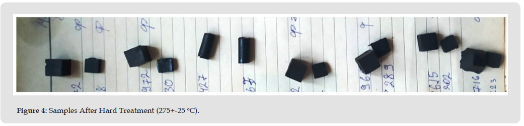
It is important that we do not have a collapse in strength, but only a decrease in ≈1,5 times. After hard heating, all the samples are carbonized (Figure 4). But unfilled sample keeps the compression strength F at the original untreated level (Table 3). Oil samples change F in different ways. For 5P (5 wt% of refined), the indicator increases even to the level of unfilled (without warming it was much lower, … kgf/cm2). Also, the 20P sample (with 20 wt% refined oil) shows a significant increase after special heating, while the 20HP practically does not change the indicator. Such interesting effects can be called “thermostrengthening” of epoxy plastics. Regarding it, there are publications on epoxy-iron , epoxy-carbide and epoxy-gypsum compositions [7-9]. But epoxy-oil composites theoretically do not have solid microparticles, heat-resistant inclusions and other that can give such strengthening. This strange fact can be explained by the fact that weak and fast-burning inclusions disappear at 275 oC, and the polymer network has not yet destroyed, and therefore we have amplification. Obviously, this can only happen at certain optimal dilution concentrations. Indeed, at 33%, and especially at 10% dilution with both oils, heating leads to a decrease in strength.
It is interesting that after standing in a strong HNO3 solution, the influence of oils becomes positive at all taken concentrations. An unfilled sample after such exposure loses its strength more than one and a half times (from 670 to 430 kgf/cm2), as well as 20 HP and some others. However, some oil samples sometimes increased it or slightly lost it. Thus, 5P reduced F from 670 to 610 kgf, and 33HP increased it by 1.5 times(from 420 to 610 kgf). Thus, there are optimal concentrations of oil, at which we have a significant increase in resistance to a strongly acidic oxidizing environment.
Microhardness
Unfilled epoxy compositions without heating give a result of 70- 85 units (Table 4). This, for comparison, is equal to the strength of the plastic used in the manufacture of industrial protective helmets. According to my expectations, the oil should have significantly reduced this indicator due to its density, but to my surprise this did not happen. За the average value of the three measurements made for each composite, it can be observed that the oil, both refined and unrefined, gave results that are within these limits, this means that the oil has no effect on the microhardness of epoxy compositions in such proportions According Table 4, the oil has stronger effect on the microhardness of epoxy compositions, that increases to 10-15%.
Table 4: Microhardness of unheated composites.
Conclusion
1. This work is relevant in wide industrial sectors, due to the reduction in the price of the final solidified biocompatible material. This is confirmed by a number of modern publications in the scientific literature.
2. The compositions “epoxy resin – vegetable oil” can be obtained in a fairly wide range of concentrations, up to 35% by weight of oil. Further filling carries the risk of phase separation in the mixture, and this is more likely for refined than for unrefined. It was also noticed that at medium and high contents (20-33%) unrefined oil gives visually more solid composites (yellow in color), while refined oil forms an oil layer separated from the composition on surface of the samples. Optical microscopy shows that the introduction of oil leads to the appearance of large drops-inclusions of oil in the epoxy-oil emulsion.
3. Also, it was established that all oil-diluted samples (after normal treatment at 70-80°C) show a noticeable (in ≈1.5 times) decrease in compressive strength. This decrease depends little on the concentration and refinement of the tested oil. This can be explained by the softening effect of oil inclusions. However, after severe heat treatment (275 oC) unfilled loses his strength, but some oil samples (with 5-10% refined oil) can significantly increase compressive strength, or do not change it (with 20% unrefined). Even more clearly, this effect of strengthening after aggressive influences is manifested after exposure to a strong solution of nitric acid, where the unfilled sample loses its strength by 1.5 times, and some oil samples do not lose strength much (with 5% and 33% raf. and with 10% unrefined) or significantly increase it (from 33.5% unrefined). These effects may indicate an important stabilizing role of oil inclusions during extreme actions.
4. Based on all the obtained data, the author’s model scheme of the formation of the epoxy-oil mixture is presented, as well as the possible placement of inclusions and inhomogeneities in it. It partially explains the effects of the different action of refined and unrefined oil in the composition with epoxy resin.
5. The obtained results allow us to talk about the high prospects of creating such compositions to reduce the price of epoxy materials, improve their biocompatibility, resistance to aggressive influences, and increase some important strength indicators.
6. According the obtained data, the author’s model scheme of the formation of the epoxy-oil mixture (and possible placement of inclusions and inhomogeneities in it) is presented. It partially explains the effects of the different action of refined and unrefined oil in the composition with epoxy resin.
7. The obtained results allow us to talk about the high prospects of creating such biocompositions – for reduce the price of epoxy materials, improve their biocompatibility, resistance to aggressive influences, and increase some important strength indicators.
Structural Fiber Mesh Reinforcement of a Polymeric Heart Valve: Improving Valve Durability and Leaflet Closure Effectiveness
Introduction
Valvular heart disease is an illness caused by damage to human heart valves. A human heart has four valves: the aortic, mitral (bicuspid), tricuspid, and pulmonary valves. These valves facilitate the controlled flow of blood through the heart. Thus, damage to the valves, caused by calcification, endocarditis, rheumatic disease, and congenital heart valve disease, have devastating effects on health. To treat valvular heart disease, patients must undergo valve replacement surgery, where a prosthetic heart valve is used to replace the diseased heart valve. There are two main prosthetic heart valves used today: mechanical and bioprosthetic. Mechanical heart valves are mostly made of stainless steel or titanium with leaflets of pyrolytic carbon with graphite coating [1-5]. While very resilient, mechanical heart valve replacements create high amounts of shear stress upon the blood, causing excessive coagulation, which requires patients to undergo a lifetime of therapeutic anticoagulation to reduce thrombus formation and stroke [6-8]. Meanwhile, bioprosthetic heart valves are made of bovine and porcine pericardium sewn to frames. These alternatives maintain the shape of native heart valves and are largely hem compatible, significantly lowering the risk of thrombosis and the need for anticoagulants in patients. However, bioprosthetic valves deteriorate over time because of the body’s immunological response which causes calcific degeneration upon the valve. Eventually, the patient must undergo another replacement valve within 15 years, making bioprosthetic valves non-viable for younger patients [9].
Moreover, bioprosthetic valves cannot be mass-produced, and animal pericardium is not a readily available resource, making it challenging to produce bioprosthetic valves at its demanded rate. As both mechanical heart valves and bioprosthetic valves have significant drawbacks, alternative valve replacements have gained significant interest. The principal among them are polymeric valve prostheses, which are capable of combining the mechanical durability of mechanical heart valves and the hemocompatibility of bioprosthetic valves [10-12]. Yet, polymeric valves continue to present concerns which make only a select few viable. Particularly, thrombotic complications can be provoked by changes in the hemodynamics along the valve. Indeed, the rigidity in leaflet materials and certain valve designs create high shear stresses upon the blood, leading to hemolysis, platelet activation, and ultimately thrombosis. However, modern polymeric valves have developed a tricuspid design that minimizes shear stress and damage to red blood cells, reducing thrombosis [13-15]. The properties of the polymer itself have a significant effect on thrombus formation as well. Interactions between the blood and the polymer often led to the absorption of proteins upon the surface of the leaflets due to a variety of chemical properties of each polymer. A number of these proteins (Fibrin, clotting factors) in turn stimulate platelet activation and coagulation, which commonly lead to thrombosis [16-19]. Thus, it is important that the polymers chosen have desirable chemical properties to reduce the risk of thrombosis.
Calcification, additionally, may also induce failure in unsuitable polymeric heart valves, as calcium deposits restrict leaflet mobility and lead to regurgitation and valve failure [20-22]. Some rigorous long-term in vivo tests showed that the issues such as inflammation along the valve, polymers accelerating the mineralization process, and the accumulation of blood proteins and phospholipids can accelerate the calcification process and cause even earlier valve failure. Particularly, polyurethane (PU)-based valves and expanded polytetrafluoroethylene (ePTFE) valves demonstrated issues with calcification due to calcium deposits building up in the porous structure or in cracks in the polymer to reduce flexibility [20-22]. Another main factor for polymeric valve failure is the degradation of the polymeric leaflets due to both mechanical and physiological factors. Polymers used for heart valve leaflets must possess sufficient tensile strength, flexibility, and fatigue resistance, enough to survive constant pressures of up to 1 MPa experienced by the leaflets [23,24]. To withstand these pressures, native heart valves are capable of withstanding pressures of approximately 2 MPa, which is further supported by the regenerative ability of native valves [25,26]. However, replacement valves are thought to need a significantly larger tensile strength due to their inability to recover. For example, bioprosthetic valves have tensile strengths of over 10 MPa. As a result, a large number of polymers (polyetheretherketone, etc.) are immediately unsuitable by themselves due to their inferior elasticity and strength, despite their biocompatibility.
Of similar importance, the leaflets of polymeric valves must also have sufficient fatigue and creep resistances to withstand the cumulative effect of countless loading-unloading cycles and resist deformation. Then, polymers like polyethylene are less viable alone due to their weak intermolecular bonds causing deformation over time [25,27,28]. Additionally, the physiological processes of the human body can degrade the polymer due to interactions with water, ions, proteins, and lipids in the body. These different molecules in turn lead to changes in mechanical properties in the leaflets (plasticization among others), leading to eventual failure [25,29]. Particularly, hydrolysis and oxidation create biodegradation in many polymers [30, 31]. To satisfy these various requirements for polymeric heart valve replacements, in this paper, we present a novel approach fiber-reinforced polymeric heart valve replacement, which utilizes additional structure to provide greater support. Polydimethylsiloxane (PDMS) has been observed to reduce calcification in heart valves [32]. PDMS is a polymer with well-proven, high hemocompatibility, biostability, and good elasticity, which is used today in a variety of biomedical applications ranging from aneurysm grafts to coating implantable devices and is the most frequently utilized polymer in implantation devices. Due to these qualities, using PDMS in polymeric heart valves is expected to reduce thrombus formation and calcification on the polymer’s surface, highly desirable attributes for heart valves.
Despite its superior biocompatibility, PDMS is largely regarded as a suboptimal material for polymeric heart valve leaflets due to its unfavorable mechanical qualities for a heart valve. However, PDMS has a tensile strength between 2.2 and 6.7 MPa [33], which presents concerns regarding the valve’s ability to withstand the pressure of blood flow over extended periods of time. Additionally, although PDMS is considered to have relatively decent fatigue resistance, it presented significant structural degradation under long term testing in heart valve leaflets [33]. To overcome this problem, PDMS grafting on the surface of polyurethane leaflets was recently tested, where the increased hydrophobicity of the PDMS was seen mitigating the calcification process significantly. On the other hand, imperfections in the grafting process made the graft degrade over time, leading to the same concerns with physical degradation seen in normal polyurethane valves [34]. To circumvent issues concerning grafting, this study obtains inspiration from the optimal structure of the native heart valve. In native valve leaflets, there are three primary layers: the fibrosa, spongiosa, and ventricularis layer, as shown in Figure 1a. The outermost fibrosa layer is composed of collagen fibers, which provides structural strength to the leaflet under higher stress, taking the load off the weaker spongiosa and ventricularis [35-37]. Beneath it, the spongiosa layer consists of polysaccharide compounds so that it maintains flexibility and provides additional support under lower load.
Figure 1
The innermost ventricularis layer consists of endothelial cells and provides the valve with its hemodynamic properties, preventing clot formation and reducing shear stress. Figure 1b shows a perspective view of the aortic heart valve leaflets mimicking the natural fiber structure. Imitating the optimal design of native valves – fiber embedded flexible matrix – can eliminate the issues with grafting PDMS. This study investigates fiber reinforced PDMS leaflets as an alternative to grafting solutions. First, we describe the fabrication process of the fiber reinforced PDMS leaflets. Then, PDMS leaflets reinforced with various fiber meshes were fabricated, and their mechanical performances were tested in vitro.
Materials and Methods
Leaflet Design
The given polymeric heart valve leaflets consist of three layers: the fiber mesh layer in between the PDMS matrix layers. The fiber mesh layer has an evenly spaced grid of nylon fiber of a specified thickness embedded within the PDMS matrix. The density of the grid is determined by the thickness of the fiber – thinner fibers have denser grids. In this study, fiber meshes of three different thicknesses were manufactured to demonstrate the customizability of the fiber mesh: 100, 350, and 600 micrometers. The heart valve proposed herein is imitating a triscupid valve, and the fiber reinforced polymeric leaflets are designed to have an elliptical semilunar shape. The semicircular edge of the leaflets were sewed onto the top part of the valve to create stability and easy attachment.
Forming the Fiber-Reinforced PDMS
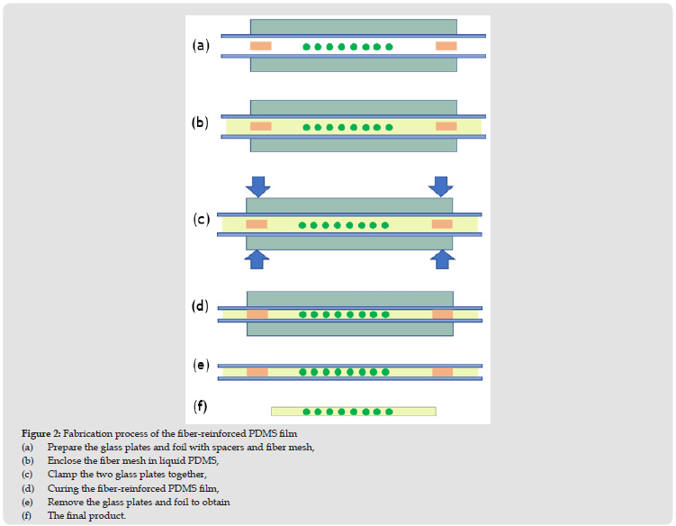
Figure 2 shows the fabrication process of the fiber reinforced polymeric leaflets. Two 4-inch by 4-inch glass plates and four spacers are prepared as mold for the leaflets. Both glass plates are covered with aluminum foil to make the removal process easier and ensure that both pieces of glass have no remaining debris. The thickness of the composite leaflet is controlled with four spacers that are placed between the two glass plates (Figure 2a).
To create the PDMS matrix, the Dow Corning Sylgard 184 silicone elastomer kit including both a silicone elastomer base and a curing agent is utilized. The ratio of the silicone base to curing agent is 10:1, and the elastomer is carefully mixed for 10 minutes. Before curing, the liquid PDMS is placed into an air vacuum to remove air pockets generated during mixing and to create uniform silicone leaflets. The prepared fiber mesh is put in a container, then a sufficient amount of the liquid PDMS is poured in the container to fully wet the fiber mesh. The wet fiber mesh is placed into the air vacuum to remove air pockets between fibers. The liquid PDMS is also poured on both glass plates to form the top and bottom matrix layers.
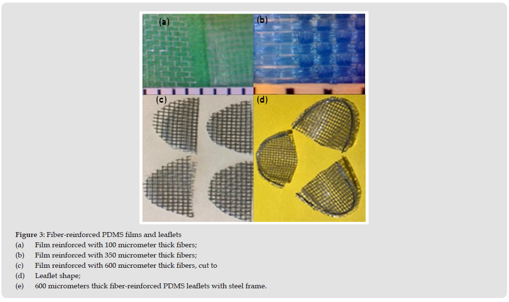
When the air pockets were removed, the PDMS covered fiber mesh is sandwiched between 2 glass plates as shown in Figure 2b. Then, the glass plates are clipped together (Figure 2c) so that the gap between the glass plates has the thickness of the spacer. The fiber reinforced PDMS in liquid phase is cured into a solid by heating at 135℃ for 30 minutes (Figure 2d). After the PDMS liquid has formed into a soft silicone, the fiber mesh film is left to cool to room temperature before prying away the foil and glass plate to create the elastomer (Figures 2e & 2f). In this final step of removing the glass plates and foils, caution should be taken to retain the elastomer’s form prior to manipulating the shape and structure. These leaflets are shown in Figures 3a & 3b, respectively.
Figure 2
Fabricating a Polymeric Valve
Using a size guide, the fiber reinforced PDMS film is cut into the shape of semicircles (Figure 3c). To make a frame for the leaflet, 8 inches of stainless-steel wire, with a diameter of 1.0 mm, is cut, straightened, and folded in a way in which the wire is parallel with itself, but one half is slightly longer than the other. The cut fiber mesh film is placed between the steel wire so that the folded portion is tightly hooked perpendicular to the arcuate edge of the semicircle. Then the wire is gently manipulated to follow the arcuate edge all the way around, leaving. 1.0 mm of space between the wire and the arcuate edge on both sides of the fiber mesh film (Figure 3d). Then a 2- inch piece of thin stainless-steel wire (0.3 mm diameter) is utilized to stitch the steel wire frame to the silicone leaflet. Similar to the thicker steel wire frame, the 0.3 mm wire is folded to where one half is a centimeter longer than the other. Then, following the guide of the thicker steel wire, the 0.3 mm thin wire is punctured through the fiber mesh film ensuring that the 2 different halves of the wire are on opposite sides of the thick wire frame. Once the 0.3 mm wire has been pulled secured, the two thin wires are twisted using pliers. The twists should be tight and about 2.0 mm long, any excess is then cut. Continue this cycle of stitching with the 0.3 mm wire 4 more times for a total of 5 stitches evenly dispersed throughout the arcuate edge of the silicone leaflet. As a final step, the thicker 1.0 mm wire, acting as the frame of the leaflet, is cut to line up with the end of the flat edge perpendicular to the arcuate edge, and the slightly longer half on the parallel side of the silicone leaflet is bent using pliers to enclose the frame-like structure.
Figure 3
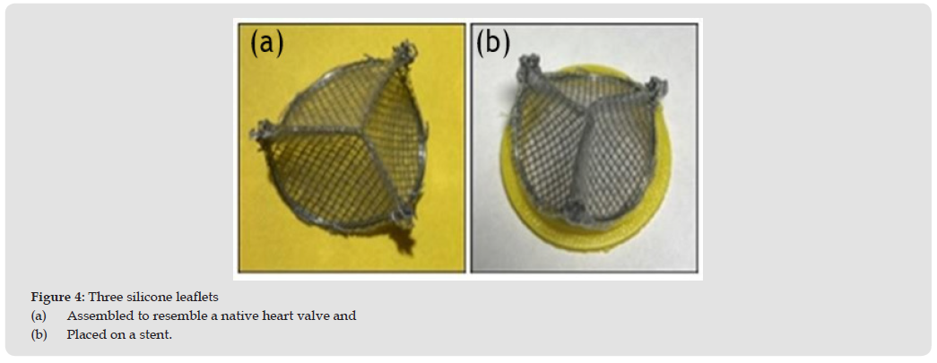
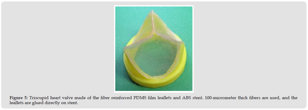
This process is repeated to create a total of three uniform leaflets all with the same wire structure, and finally the three leaflets are arranged in a form resembling a native heart valve, stitched to secure proper commissure points, placed on a short stent, and glued onto the arcuate edge of the leaflets, beginning slightly below each commissure point (Figure 4). Alternatively, the fiber reinforced PDMS leaflets may also forgo the use of stainless wire for stability altogether and, instead, use a slightly taller stent. In this configuration, after the artificial leaflets with PDMS and fiber mesh are created, the leaflets’ arcuate edge is immediately glued to the altered stent to simplify the manufacturing process (Figure 5). The commissure points are formed at the corners of each leaflet as in the other manufacturing process; however, the leaflets will be glued together instead of sewn together with wire. Additionally, the leaflets may also be sewn to the stent instead. The stent is made of acrylonitrile butadiene styrene (ABS) and fabricated using a 3-D printer.
Figure 4
Figure 5
Experimental Set-Up
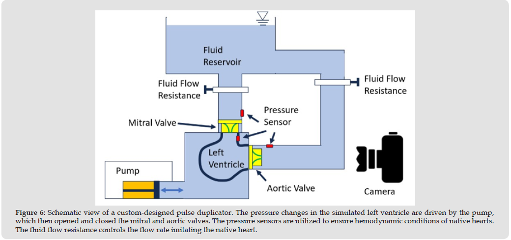
The hemodynamic performance of the fiber-reinforced polymeric heart valve created using the fabrication method was tested in vitro to verify its performance in a pulse duplicator. Figure 6 shows the conceptual view of our custom-designed pulse duplicator. For testing, two heart valves with 100-micrometer thick fiber-reinforced leaflets glued directly onto the stent without a metal wire structure (Figure 5) were placed onto the pulse duplicator simulating a mitral valve and an aortic valve. The pulse duplicator was then set to imitate the hemodynamic conditions of the native heart valve with a forward pressure of 100 mmHg across the valves, created by the pump. The fluid flow resistors maintain an average flow rate of approximately 5 liters per minute.
Figure 6
Results
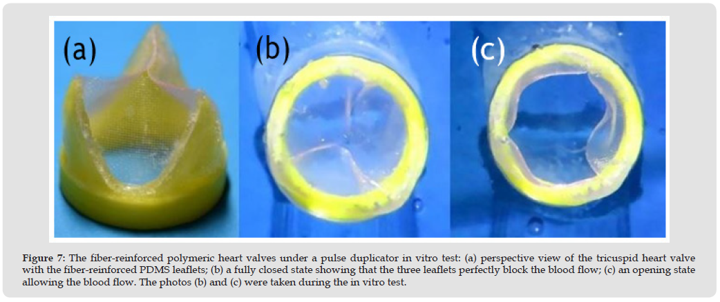
In the in vitro pulse duplicator test simulating blood flow in hearts, the fiber reinforced PDMS valves demonstrated promising hemodynamic behavior. Both valves demonstrated sufficient leaflet functionality: the valves opened and closed properly without any issue and responded quickly to changes in pressure caused by the pump. The valves appeared to be stable and entirely functional over repeated cycles with full opening and closing each cycle, indicating that the insertion of a fiber mesh layer does not significantly hinder the flow rate or cause regurgitation. Furthermore, the possible viability for long-term use is indicated. The valve leaflets did not undergo plastic deformation and maintained their physical properties after the tests, which demonstrate that the suggested fiber reinforced PDMS leaflets are capable of withstanding the mechanical conditions of the heart. Among the leaflets reinforced with three different fiber thicknesses, the leaflet reinforced with 100- micrometer thick nylon-mesh showed the best functionality during the opening and closing cycles as shown in Figure 7. Therefore, the leaflet reinforced with 100-micrometer thick nylon-mesh can be used for heart valve replacements without concerns regarding effective orifice area and regurgitation and with hopes of long-term structural integrity.
Figure 7
Discussion
A sufficiently high strength is one of the essential requirements of successful polymeric heart valve to maintain the functionality of the leaflet under high-pressure conditions. As aforementioned in Figure 1b, in native heart valves, the high strength is accomplished by circumferential collagen fibers in the leaflet. In the polymeric heart valve proposed herein, the fiber mesh placed within the PDMS matrix plays the role of the circumferential fibers of the native heart valve. The strength of nylon is 85 MPa while that of PDMS is 3-5 MPa, and the insufficient strength of PDMS can be complemented by the nylon reinforcement. The composite strength can be adjusted by changing the density of fibers in the cross section. The fibers reinforcement can prevent the surrounding PDMS matrix from excessive strain, and correspondingly, the normally weak PDMS leaflet’s fatigue resistance increases and, structural damage of the PDMS matrix is prevented. Thus, by adding this additional layer of support to the leaflet, the mechanical properties of the PDMS layer are favorably altered to allow for use in heart valve leaflets. On the other hand, a successful heart valve leaflet should have the ability to stretch under relatively low strain conditions within the heart. Within native valves, the low Young’s modulus (0.3–1 MPa) and high ductility (strain of 150%) of the elastin in the ventriculitis layer provides high flexibility, allowing the valve to open and close easily in normal condition [38]. In terms of flexibility and ductility, PDMS is a perfect material mimicking the behavior of natural heart valve leaflets because PDMS has similar Young’s modulus (0.36–0.87 MPa) [33] and ductility (~140%) [39].
Although the Young’s modulus of nylon fiber is very high (0.5-3 GPa), the effect of the fiber mesh on the flexibility can be eliminated by aligning the fiber mesh in diagonal direction to the circumferential direction (the direction of maximum strain) of leaflets. The collagen fibers in natural heart valve leaflets also have diagonal alignment as shown in Figure 1b. Under low-pressure conditions, the flexibility of leaflets is a critical factor for the functionality of heart valves [40]. The fiber reinforced PDMS leaflets are highly customizable due to the fabrication method. The mechanical behavior and the life of the proposed leaflets can be engineered by adjusting the type, grid density, thickness, and direction of the fibers. These possible modifications also ensure the ability to further optimize the current design in future iterations. The thickness of the PDMS matrix is also customizable, allowing for fine- tuning of the valve’s mechanical behavior. Furthermore, the simple customizability of each leaflet allows for a variety of possibilities in optimizing the leaflets’ mechanical integrity and hemodynamic interactions by changing the mechanical properties of each leaflet. To provide additional structural stability to the leaflets, the fabrication process of the proposed valve utilizes a metal support wire along the arcuate edge of the leaflets. This added structure is expected to significantly improve the structural integrity of the leaflet along the edge attached to the stent by glue. More significantly, the stiffer support wire allows for much simpler attachment between the leaflet and valve stent, as the arcuate edge is stiffer and easier to maneuver, reducing the risk of manufacturing errors.
This wire- framed fabrication allows the fiber-reinforced polymeric heart valve to be clampable on a catheter and can be used for Transcatheter Aortic Valve Replacement (TAVR) [41,42]. Although TAVR is one of leading medical procedures in this field, this article is focused on the fabrication of the fiber-reinforced polymeric leaflets assuming regular heart valve replacements. However, it should be noted that the fiber-reinforced polymeric heart valve has potential for being optimized for TAVR through future work. An additional benefit of using PDMS for heart valve leaflets is the hydrophobicity of PDMS. The hydrophobic leaflet surface decreases the shear stress caused by the blood flow through the heart valve and eventually reduces the thrombogenicity of the valve. This then removes the necessity for the prescription of anticoagulants for patients. Moreover, the superior biocompatibility of PDMS, which only causes minimal inflammation for a short period after insertion, significantly reduces the amount of calcification occurring on the leaflets by reducing the body’s immune response to the foreign polymer, and eventually increases the valve’s longevity and structural integrity compared to other biomechanical valves. Also, the increased fatigue resistance, achieved by the fiber-reinforcement, reduces long term structural valve degradation, and increases the life of the valve.
Conclusion
An artificial heart valve made of fiber reinforced PDMS leaflets that has advantages over conventional mechanical and bioprosthetic valves is suggested, and its fabrication process is proposed. The hemodynamic performance of the fabricated composite valves with fiber reinforced PDMS leaflets were successfully validated through short-term in vitro tests under cyclic flow generated by a pulse duplicator. PDMS has excellent hemocompatibility and biocompatibility but is not a favorable polymer for heart valve leaflets because of its weak strength. However, the shortcoming of PDMS can be eliminated by embedding the fiber mesh reinforcement layer that is inspired by the collagen fibers of natural heart valves. The suggested leaflet fabrication process is simple and has potential to be customized through selection of fiber, grid density, and fiber alignment. Thus, customizability of the valve leaflets allows for the optimization of the given design and thus shows great promise. The mechanical durability of the fiber reinforced PDMS valve is expected to be superior due to the reduced stress in PDMS matrix. For further investigations, interactions between the valve and blood, particularly regarding calcification and thrombus formation, are suggested as a follow-up test with a long-term experimental setup. While the PDMS matrix is expected to reduce calcification, it needs to be confirmed whether certain protein interactions along its surface may induce undesirable calcification.
Furthermore, the effects of various modification factors such as fiber type, direction, mesh density, leaflet thickness, and wireframe on the mechanical behavior need to be investigated for the optimization and TAVR application of the fiber reinforced PDMS. In conclusion, the optimistic results of the in vitro pilot tests for the proposed design shows that the proposed fiber-reinforced PDMS valve is promising in the context of finding a biocompatible, durable, and cost- efficient alternative to the current mechanical and bioprosthetic valves and opens many exciting avenues for further research.
Acknowledgements
This work was conducted with the support of the University of Texas Rio Grande Valley.
Drug use Evaluation on Magnesium Sulfate use in Obstetrics Wards: the Case of Ras Desta Damtew Memorial Hospital 2023 GC
Introduction
Background
Hypertension is a common medical problem that complicates pregnancy. It may be, manifested as chronic hypertension, chronic hypertension with super imposed preeclampsia, Pregnancy induced hypertension, preeclampsia or eclampsia. Hypertensive disorders in pregnancy can be manifested by increased blood pressure(BP) greater than or equal to 140/90 mmHg during pregnancy. Measured four hours apart and after 20 week of gestational age. The presence of the other clinical symptoms and signs of hypertension in pregnancy depends on the severity of the disease. Pre-eclampsia (PE)is part of pregnancy induced hypertension(PIH) which is defined as a BP > 140/90mmHg in the presence of significant proteinuria of greater than 300 mg per 24 hours urine Specimen or, less accurately, more than 1+ protein (equivalent to Approximately 100mg/dl) on dipstick in at least two randomly collected Urine specimen at least 6 hours apart after the 20th week of gestation or up to 6 weeks postpartum. Preeclampsia with severity features (Sever Preeclampsia) is the presence of Diastolic BP > 110 mmHg and the systolic BP ≥160mmHg measured twice at least six hours apart or a single measurement of >120mmHg, Hyperbilirubinemia, Hemolytic anemia, Thrombocytopenia (Less than 100,000/μL), Elevated Liver Enzymes (HELLP syndrome), Disseminated Intravascular Coagulation (DIC), Headache, visual disturbance and right upper abdominal pain, Oliguria ( less than 400ml in 24hours or 30ml/hour), Cardiac decompensation, pulmonary edema, cyanosis, Exaggerated Deep Tendon Reflexes (DTR).
Eclampsia is the occurrence of convulsions in woman who meets the diagnostic criteria for pre-eclampsia. Any convulsion occurring during pregnancy is eclampsia unless Proven otherwise. Anti-convulsants such as Magnesium Sulphate (MgSO4), as well as antihypertensive medication, are rarely required for patients on conservative management (mild preeclampsia). Delivery is the definitive treatment for mother with sever preeclampsia. The primary objective is to prevent convulsion, intracranial bleeding and other vital organ damage. MgSO4 is one of the main interventions used to decrease the morbidity and mortality from preeclampsia/eclampsia. In 2011, MgSO4 has been strongly suggested by the World Health Organization (WHO) to be the drug of choice for both treatment and prevention of eclampsia. Ethiopian Food and Drug Authority also recommends this; loading dose of 4gm as 20% solution IV over 10-15 minutes followed by 10gm as 50% IM injection divided on two sides of the buttock, followed by maintenance dose of 5gm every 4 hours as 50% concentration over 2minutes, 2gm IV as 50% solution over 2minutes if convulsion recurs. And, reduce the maintenance dose by half if there are signs of renal impairment during labor and for the first 24 hours postpartum. Adverse Drug Effects associated with the use of MgSO4 can be Respiratory Paralysis, pulmonary edema, depressed tendon reflexes, hypotension and hypocalcaemia. Therefore, renal function, BP, respiratory rate(RR), and DTR should be monitored when MgSO4 is administered parenterally. Hypersensitivity, myocardial damage, diabetic coma, hypermagnesemia, hypercalcemia, and administration during 2 hours preceding delivery for mothers with toxemia of pregnancy. In patients with renal impairment it has to be ensured that renal excretory capacity is not exceeded by halving the recommended dose.
Significance of the Study
The findings from this study could fill the gap in the obstetric use of MgSO4 in the management of PE/E. This would identify problems in MgSO4 use and suggest for further studies by researchers and healthcare facilities.
Methodology
Study Area and Study Period
The study was conducted in Obstetrics wards of Ras Desta Damtew Memorial Hospital (RDDMH) from october 1 2022 to september 30,2023 G.C. The hospital was established in 1924 E.C. RDDMH is located in Addis Ababa, Ethiopia. It has Medical, Surgical, Obstetrics and Gynecology, and Pediatrics services. In addition, there are ENT, Dental, Ophthalmology, ART, TB treatment and follow up services.
Study Design
A retrospective cross-sectional study design was used.
Study Population
All patients who received MgSO4 for the management of PE/E. Sampling Technique and Sample Size Determination Purposive sampling technique was used and 240 patient charts were collected, organized and sorted based on their MRN and according to WHO recommended sample size (75-100) for performing hospital DUE,100 charts were selected by systematic random sampling technique. From the 100 charts, 13 were excluded because there was no documentation of MgSO4.
Data Collection Procedures
Before commencing to data collection permission was received from the hospital Drug and Therapeutic Committee (DTC). Data was collected by two DUE trained personnel. The tool was adopted from Ethiopian National Medicine Use Study Guideline, 2021. And customized to our study objective. Data was directly filled on to MS-Excel data base.
Data Processing and Analysis
Data cleaning was performed after which it was imported to IBM SPSS Statistics Version 21.
Limitation of the Study
The limitation of the study was that it did not address the frequency of MgSO4 administration and control of seizure frequency. And it did not address the consumption of MgSO4 vials.
Results
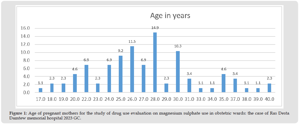
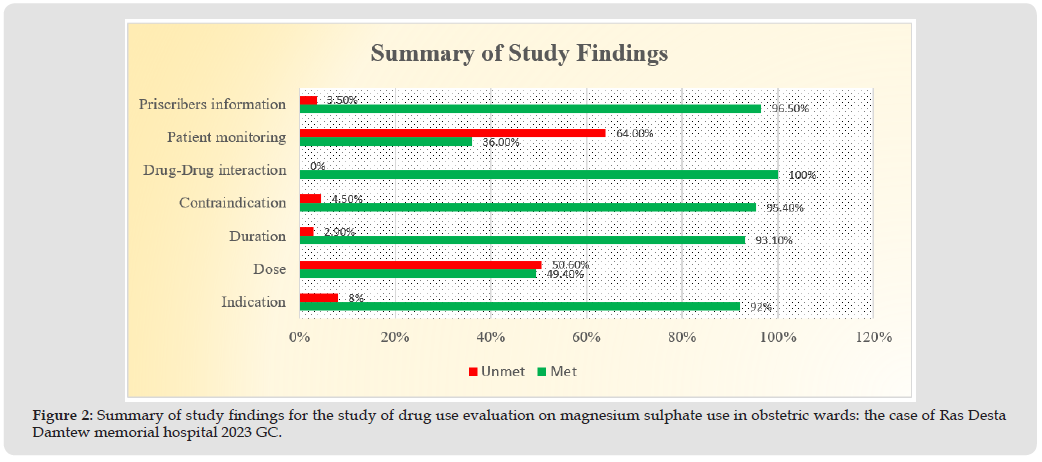
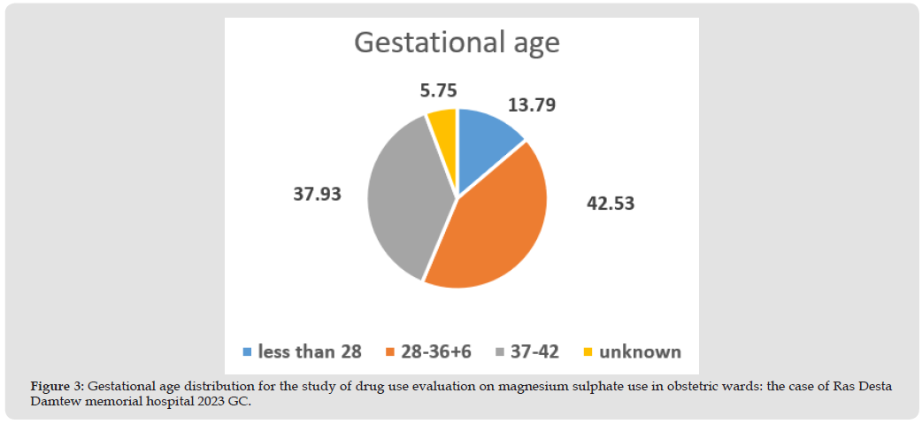
As shown in Figure 1, From 87 patient chart reviewed the minimum age of mothers was 17 and the maximum age was 40 years with median age of 27 years. And 26.5% of the mothers were within the range of 15-24 years of age, the majority of mothers were within the range of 25-34 years of age (61%) and the remaining 12.5% of mothers were within the range of 35-40 years of age. From the total charts reviewed only 16.1% of the charts had a documentation of the mothers’ weight. When the pregnancies are classified based on gestational age; 13.8% were less than 28 weeks, 42.5% were in the range of 28- 37 weeks of gestation, 37.9% were in the range of 37-42 weeks, and there were no pregnancies above 42 weeks of gestation. And 5.7% of the pregnancies were of unknown gestational age by date or estimation. 41.4% of the mothers in this study were primigravida while the rest 58.6% were multigravida. From the total charts reviewed 5.7% of the mothers had previous history of pre-eclampsia/eclampsia and 1.1% had concomitant disease which was Gestational Diabetes. The diagnosis of mothers in the study period were categorized in as mild pre-eclampsia, sever pre-eclampsia and eclampsia which were 9.2%, 83.9% and 6.9% respectively. There was no mother who developed eclampsia after admission. 80(92%) of the mothers had an indication. (5.7%) mothers were assessed to have pulmonary edema and all of them were given Furosemide injection. As shown in figure 2 below, 21 (24.1%) of the mothers were Nifedipine co-administered with MgSO4 from which none of them had developed a drug-drug interaction (Figures 3 & 4).
Figure 1
Figure 2
Figure 3
Figure 4
This was assessed by BP monitoring of the patients obtained from the pre-eclampsia/eclampsia monitoring chart. There were 4(4.6%) patient with renal impairment were being administered MgSO4. There was no record of adverse drug reaction/toxicity developed due to MgSO4. It was found that 49.4% of mothers had a documented dose of MgSO4 as per STG. From the total 87 mothers 81(93.1%) of them were given MgSO4 with the STG recommended duration (24-48hrs). Urine output and DTR were monitored for 82(94.3%) and 37(42.5%) patients respectively. While Respiratory rate was monitored for all mothers. 85(97.7%) of the mothers were improved while 2(2.3%) got worsened and referred to a tertiary hospital.The assessment of Prescriber’s information showed that prescribers full name and qualification were written in 86(98.9) and 85(97.7%) respectively. While signature and date of prescribing were recorded in all of the charts.
Discussion
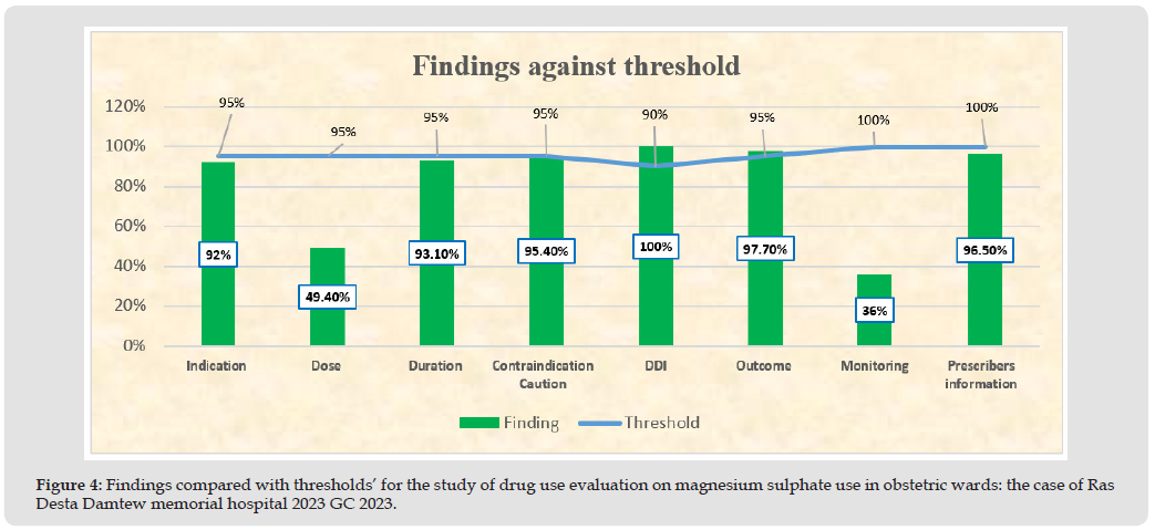
Being pregnant at age 35 or more is one of the highest risks of developing PE/E. A study done at Omdurman Maternity Hospital at Sudan showed the 25–34 years of age was the largest age group of women with preeclampsia/eclampsia. Our study result also showed that mothers between age 25-34 were the largest group of women with PE/E which is 60.7% (Alsiddig Y, et al. [1]). Body weight is strongly correlated with progressively increased PE risk, ranging from 4.3% from women with body mass index(BMI) below 20 kg/m2 to 13.3% in those with a BMI over 35 kg/m2 (Knight et.al, 2010). In our study the weight of mother was recorded only for 16.1%. This shows that there is a gap in the identification of risk factors for Preeclampsia by healthcare providers during ANC [2]. The study finding revealed that only 5 of the mothers had previous history of PE/E which can be the risk factor for developing recurrent PE/E and on which magnesium sulphate can be administered as a preventive therapy and all of those mothers were given MgSO4. From the findings of the study it can be concluded that most of the mothers were diagnosed with severe PE (83.9), while only some of them were diagnosed with mild PE and E (9.2% and 6.9% respectively). From the total mothers 80 (92%) were found to have appropriate indication for MgSO4. This finding is below our set threshold which was 95%. So 7 mothers took MgSO4 without indication, this includes those who were given MgSO4 for mild PE which is not recommended and also it can be due to patients who were given MgSO4 who did not fulfil the criteria for preventive therapy of PE/E [3].
Only 49.4% of the mothers took appropriate dose of MgSO4 as recommended by the STG which is much deviated from the set threshold 95%. This does not mean that those mothers did not take the recommended dose because this study did not assess that, but on the patient charts physicians did not record the recommended dose correctly on the order sheet. They just order it ‘as per protocol’ which is not correct. Even if the dosing protocol is found in the obstetric wards of the hospital, it is mandatory to write the loading and maintenance of MgSO4. This was a great obstacle which made it difficult for us to know the exact quantity of MgSO4 the patient took. Only 4(4.6%) of the mothers had renal impairment while 83 (95.4%) of them did not have renal impairment. This result is above the set criteria for contraindication of MgSO4 administration which was 95%. MgSO4 contraindication in pregnant mother not an absolute contraindication.
There needs to be dose reduction by half. It was written on the order sheet as ‘reduce the recommended dose by half’ but we did not find the exact dose administered on the medication sheet. The drug-drug interaction between MgSO4 and Nifedipine is moderate (not significant). When Nifedipine is given with MgSO4 has a synergistic physiologic effect which is hypotension which needs close monitoring of BP. The result of the study showed that 21 (24.1%) of the mothers were Nifedipine co-administered with MgSO4 [4]. They were assessed for reduced BP, from which none of them developed a drug-drug interaction. so the result is 100% which is greater than the set threshold which was 90%.
The outcome of treatment showed that 85 (97.7%) of the mothers were discharged improved. While only 2(2.3%) mothers got worsened and refereed to tertiary hospital. This finding is above the set threshold which was 95%. This result shows that MgSO4 is an effective choice of medication for the control of seizures in PE/E. Urine output and DTR were monitored for 82(94.3%) and 37(42.5%) patients respectively. While Respiratory rate was monitored for all mothers. On this study we found that a significant drawback exists in the monitoring of patients taking MgSO4. Mothers monitored for all the three parameters were 36(41.4%) which is below the set 100% threshold. The assessment of Prescriber’s information showed that prescribers full name and qualification were written in 86(98.9%) and 85(97.7%) respectively. While signature and date of prescribing were recorded in all of the charts [5]. Orders with all the four parameters recorded were 96.5% which is below the set 100% threshold.
Conclusion and Recommendation
• The study findings revealed that documentation of mother’s weight was poor; where weight(BMI) increment is a significant risk factor for PE/E. there for we strongly recommend the measurement of pre pregnancy or first ANC weight (BMI) [6]. • Indications for MgSO4 administration was found appropriate for most of the mothers, but there were mothers found taking MgSO4 against STG recommendations. However, it is ultimately the decision of the attending healthcare providers to start MgSO4. • The dose of MgSO4 was not recorded correctly on order sheets, so we recommend physicians to write the full recommended loading and maintenance dose and also we recommend nurses to record each administered doses of MgSO4 including the route. • Overall the correct dose of MgSO4 is not recorded obstetric order sheets [7]. • It is recommended that the duration of MgSO4 to be 24-48 hours as per STG. We found some gaps only on some mothers who were given MgSO4 below and above this duration, so it may be due to documentation gap, mothers response to treatment or duration of seizures. We strongly recommend for a complete documentation of MgSO4 duration of administration. • Since there is a gap in monitoring of patients and recording on PE/E follow up chart. We strongly recommend the maternity ward staff to monitor and record Urine output, DTR and RR [8]. • Prescribers name, qualification, signature and date of prescription must be written on all orders. • We found that charts in the gynecology/obstetrics ward are disorganized which made it difficult for us to find the exact data we wanted. But now since electronic medical recording is started it may fill this gap [9].
Acknowledgement
We would like to thank our hospital DTC, Research and Training Department for the technical assistance and decisions passed on ethical procedures. We thank the Obstetrics and Gynecology Department, and Medical Record Room for their great cooperation in providing assistance and retrieval of patient charts. Our deepest gratitude also goes to Federal Ministry of Health of Ethiopia and World Health Organization for organizing the orientation and providing of the tools, technical assistance in data analysis and preparation of the final document.
Boerhavia Diffusa Linn: Unravelling the Medicinal Tapestry from Ayurvedic Traditions to Modern Science
Introduction
The Nyctaginaceae family of medicinal plants, Boerhavia diffusa Linn., is well-known in Indian traditional medicine for its therapeutic qualities. It is also acknowledged in other areas of the world and in certain countries of South America. In the context of Indian traditional medicine, it goes by several names such as Punarnava, Shothaghni, Kathillaka, Varshabhu, Raktapushpa and Varshaketu [1]. Within the context of Indian Ayurveda, Boerhavia diffusa is designated as a “rasayana” herb, believed to possess diverse qualities including anti-aging effects, enhancement of life and memory power, and disease prevention. These attributes suggest that the herb fortifies the body’s resilience against external threats, essentially offering hepatoprotection and immunomodulation [2]. In specific areas, the entire plant serves as a vegetable. For instance, in regions like Assam and West Bengal in India, local communities cook the leaves as a culinary delicacy [3]. Different types of the Boerhaavia genus can be located across tropical, subtropical, and temperate regions worldwide, spanning Australia, Asia, the United States, and Africa. Within the Indian subcontinent, B. diffusa is prevalent in warmer regions of the country, reaching altitudes of up to 2000 m in the Himalayan region [4]. Six of the forty species in this genus—B. diffusa, B. erecta, B. rependa, and B. rubicunda— can be identified in the Indian subcontinent. In particular, B. diffusa has been the subject of a great deal of research because of its chemical makeup and medicinal qualities.
The roots of B. diffusa are the source of a distinct group of isoflavonoids known as rotenoids, along with flavonoids, xanthones, purine nucleosides, lignans, and steroids. Numerous studies and trials have confirmed its diverse activities, including immunomodulation, anticancer effects, antidiabetic properties, antioxidants, and anti- inflammatory attributes. During diverse studies conducted on the B. diffusa plant, preliminary examinations have detected the existence of β-sitosterol [5], and alkaloids [6]. The root of this plant has been traditionally used by several tribes to alleviate liver disorders. Specifically in South Garhwal, the tribal community has applied the roots for the treatment of various diseases such as liver enlargment [7]. Moreover, tribes have been using the plant’s roots of ‘Punarnava’ (Boerhavia diffusa) to treat jaundice in the eastern parts of Rajasthan and Gujarat state [8,9]. Besides, B. diffusa roots are recommended in some parts of Madhya Pradesh to treat kidney and liver problems [10]. This review offers a condensed overview of the bioactive components and documented pharmacological effects, presenting an ethnopharmacological evaluation of the said plant.
Geographical Distribution
The Boerhavia genus, consisting of 40 species, is distributed across tropical, subtropical, and temperate zones worldwide. Boerhavia diffusa, or B. diffusa, is a plant that was originally native to Brazil and India but is now found in tropical, subtropical, and temperate countries with elevations of up to 1200 metres above sea level. It is found in many places, such as Mexico, Asia, Africa, the Indian and Pacific oceans, Egypt, and Sudan [11,12]. In India, six out of the 40 species within this genus can be found, namely B. diffusa, Boerhavia chinensis, Boerhavia erecta, Boerhavia repanda, and Boerhavia rubicunda. B. diffusa, specifically, is indigenous to India and flourishes in wastelands and fields after the rainy season. Furthermore, there is a limited cultivation of this plant in West Bengal [13].
Traditional Uses
As noted earlier, B. diffusa holds significant importance as a primary herbal ingredient in a variety of Ayurvedic medicinal formulations. Its incorporation in different preparations is effective in managing conditions like inflammation, jaundice, asthma, nephrological disorders, anaemia, and gynaecological issues. Table 1 categorizes several traditional formulations where B. diffusa plays a central role as a key component [14].
Table 1: Traditional formulations containing B. diffusa act as a major ingredient.
Phytochemistry
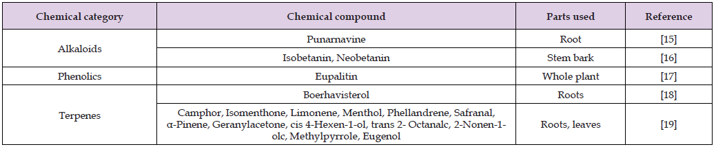
Several studies on Boerhavia diffusa species have revealed a variety of important phytochemicals across different regions, taking into account ethnopharmacological applications and advancements in technologies like mass spectroscopy, liquid chromatography-mass spectroscopy (LC-MS), Electrospray ionisation mass spectrometry (ESI-MS) etc. These investigations have unveiled significant phytochemicals in various parts of Boerhavia species, as detailed in Table 2. The conventional method for isolating compounds typically includes extraction, partitioning in different solvents, and bioactivity- guided fractionation using silica gel chromatography [15-21].
Table 2: List of chemical compounds isolated from Boerhavia diffusa.
Pharmacological Activities in Boerhavia diffusa Linn
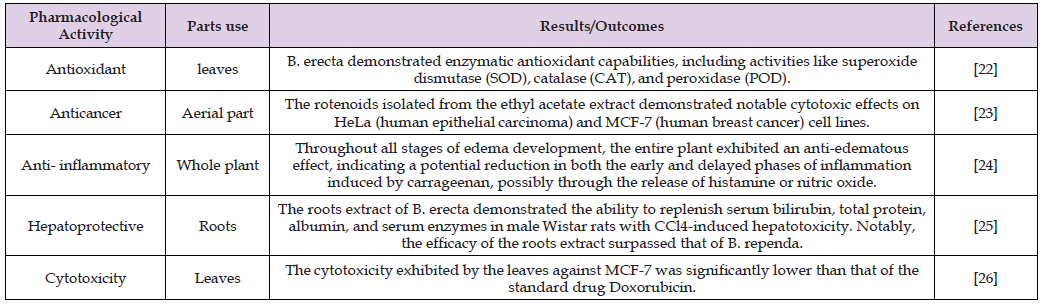
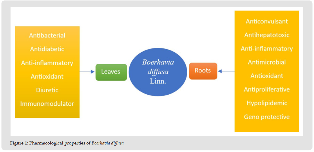
The plant Boerhavia diffusa has become significantly important in the field of phytochemistry due to its diverse pharmacological and biological activities. Various parts of B. diffusa are used in different parts of India to cure a variety of ailments. The whole plant, aerial parts, leaves, or root of B. diffusa are used in Ayurvedic herbal medicine for treating a range of medical conditions. Various pharmacological studies have shown that the plant roots of B. diffusa possess a broad spectrum of properties, including anti-inflammatory, diuretic, anticonvulsant, antifibrinolytic, antibacterial, anthelmintic, antileprotic, antiasthmatic and antistress activities (Figure 1). Table 3 compiles the available information on Boerhavia diffusa species from recent data published in the last 5-6 years [22-26].
Table 3: Various pharmacological activities and parts used of Boerhavia diffusa.
Figure 1
Antioxidant Activity
Due to its high content of tannins, phenols, and flavonoids, B. diffusa has been the subject of numerous studies examining its antioxidant potential [27-29]. The ethanolic extract of B. diffusa demonstrated the ability to scavenge 1,1-diphenyl-2-picrylhydrazyl (DPPH) radicals [28]. A fractionation guided by electron spin resonance of the methanolic extract led to the identification of boeravinone D, boeravinone G, and boeravinone H, all exhibiting significant radical-scavenging activity, with boeravinone G displaying superior antioxidant properties when compared to the other two compounds [30]. This investigation also revealed the involvement of MAP kinase and NF-kB pathways in the antioxidant effects of boeravinone G, suggesting its potential utility in injuries mediated by reactive oxygen species (ROS) [30]. In the realm of African traditional medicine, the preference for the redder stems of B. erecta prompted a study on the antioxidant potential of the redder stem bark, establishing that betacyanin’s possess greater antioxidant activity than the phenolic compounds present in the stem [31]. Similarly, the antioxidant potential of B. procumbens was attributed to its concentration of polyphenols, as demonstrated by various antioxidant assays [32]. Furthermore, B. diffusa was identified as having the capability to protect tissues from hydroxyl radical- induced DNA damage [33].
Antidiabetic Activity
B. diffusa and ethanolic extracts demonstrate notable antihyperglycemic effects in rats with alloxan-induced and streptozotocin- induced hyperglycaemia. Additionally, they show potential for improving diabetes-related conditions, as evidenced by changes in parameters such as body weight, serum cholesterol, and triglyceride levels. In recent research, the impact of streptozotocin treatment on the pancreas of diabetic control rats, along with cell regeneration facilitated by glibenclamide, was examined. Additionally, comparable regenerative effects were demonstrated through the methanolic extracts of B. diffusa [34]. An investigation was carried out on the effects of a daily oral administration of an aqueous solution containing B. diffusa L. leaf extract on the levels of hepatic enzymes and blood glucose in both normal and alloxan-induced diabetic rats over a period of four weeks. When B. diffusa L. was administered to both normal and diabetic rats, the results showed a notable decrease in blood glucose levels and a considerable increase in plasma insulin levels [35]. In rats with streptozotocin-induced noninsulin-dependent diabetic mellitus (NIDDM), the chloroform extracts from B. diffusa leaves demonstrated dose-dependent reductions in blood glucose levels. This effect was comparable to the impact of glibenclamide. These results imply that the extract’s capacity to decrease blood glucose may be linked to the regeneration of pancreatic beta cells or actions extending beyond the pancreas [36].
Anticancer Activity
The B. diffusa root and leaf extract’s in vitro cytotoxic effects show a dose-dependent response. Both the root and the leaf’s crude ethanolic extract caused 30% and 40% of the cells to die, respectively [37]. An investigation was conducted into the effect of a root extract in 95% ethanol on the growth of human peripheral blood mononuclear cells (PBMC) activated by T cell mitogen PHA and PPD antigen. The extract showed that it inhibited the proliferation of PBMCs in a human mixed lymphocyte culture as well as that induced by these stimulators. Moreover, the extract demonstrated inhibitory actions on multiple cell lines, emphasising its efficacy in experimental settings against lymphoma and leukemic cells [38]. The 95% ethanolic extract of B. diffusa root was subjected to bioassay-guided fractionation, resulting in a 30% observed cell death in the HeLa cell line. Subsequent purification through column chromatography led to the isolation of a more potent fraction. [39]. In in vivo experiments, the extract demonstrated inhibitions of 87% and 95% against metastasis both prophylactically and overall. Additionally, the survival rate of the experimental model increased by 157%. When the extract was given as a preventative intervention, serum markers linked to metastasis were reduced by 85% [40]. Furthermore, Punarnava was isolated by the author from the extract, exhibiting its capacity to trigger cytotoxicity mediated by complement and antibodies, in addition to augmenting the function of natural killer cells [41]. Numerous investigations, both in vitro and in vivo, show that a variety of plant extracts sourced from distinct plant sections may include chemicals with anticancer potential. Punarnava, an alkaloid isolated from the roots was identified and reported to possess antimetastatic properties [42].
Anti-Inflammatory Activity
The alcoholic extract of B. diffusa, which is insoluble in water, demonstrates anti- inflammatory effects in rats. Leaf and floral extracts have significant anti-inflammatory properties [43]. BD leaf extracts were tested for toxicity and for their analgesic-anti- inflammatory qualities in both juice and lyophilized decoction form. The lyophilized decoction and juice both showed about 50% reduction in abdominal writhing in mice when compared to dipyrone sodium. When compared to morphine, the juice treatment increased the mice’s latency in the hot plate test. Another noteworthy finding was the reversal of the juice’s effects following pretreatment with naloxone, except in the case of the decoction. As a result, the author suggested that the antinociceptive mechanism of the juice may be related to opioids [44]. found that BD roots contained 𝛽-sitosterol, which significantly induced swelling in mice [45]. It is commonly known that BD has anti-inflammatory qualities and is also called sothaghni, a term that denotes its ability to reduce inflammation. Most of the ayurvedic formulations mentioned in Table 1 serve purposes related to inflammation. Numerous accounts highlight the utilization of leaves, whether in their whole form, incorporated into an oral preparation, or applied topically, particularly in instances of scorpion and snake bites or for wound healing.
Antiviral Activity
Promising protective activities against potato virus X infection in both hypersensitive and systemic hosts have been observed for compounds isolated from B. diffusa L. root, Cuscuta reflexa Roxb. stem, and Euphorbia hirta L. leaves. It was found that these extracts had a systemic inhibitory effect that was actinomycin D-responsive [46]. Notable control results were obtained with the mungbean yellow mosaic illness caused by the mungbean yellow mosaic virus, which was efficiently handled by the aqueous root extract of B. diffusa. Six application sprays of B. diffusa root extract proved to be particularly efficacious, significantly delaying the onset of symptoms, mitigating symptom intensity, and reducing disease occurrence by 80-90%. In addition, enhancements in pod formation and grain output were encouraged by this treatment, along with increases in plant height, root nodulation, and primary and secondary branches [47].
Hepatoprotective Activity
Chloroform and ethyl acetate extracts were made using Bacillus cereus, an endophyte that is present in B. diffusa roots. These extracts’ hepatoprotective effects were studied in rats, with an emphasis on assessing how well they scavenged free radicals. The extract of ethyl acetate demonstrated a significant IC50 value, prompting its selection for subsequent in vivo studies [48]. The administration of endophytic bacteria extracts resulted in a normalization of the heightened levels of the aforementioned biochemicals. The findings consistently indicate that extracts derived from the endophytic bacteria of B. diffusa demonstrate antioxidant and hepatoprotective properties, ultimately leading to the conclusion. Tuberculosis presents a significant health challenge, and the primary treatment involves rifampicin therapy. While rifampicin effectively addresses tuberculosis, it is associated with liver damage. Methanolic extracts from B. diffusa leaves were investigated in the search for a natural cure. Rats were given rifampicin to induce hepatotoxicity, which resulted in a significant rise in aspartate aminotransferase, alkaline phosphatase, and alanine aminotransferase levels. In comparison to the control group, there was a concurrent decrease in serum protein levels. Studies offer proof that extracts from B. diffusa possess the ability to alleviate liver issues, attributed to the presence of flavonoids in the plant, known for their antihepatotoxic properties [49].
Anti-Arthritic Activity
Numerous research use arthritic rats to test the antiarthritic effects of extracts made from B. diffusa roots, including petroleum ether, methanol, chloroform, and water extracts. Arthritis impacted hematological factors by elevating total white blood cell counts, raising erythrocyte sedimentation rates, and diminishing red blood cell count and hemoglobin levels. Rats given extracts from B. diffusa had smaller paws and heavier bodies as a result. The recovery of red blood cells and haemoglobin, as well as the normalisation of the total white blood cell count and erythrocyte sedimentation rate, were among the several haematological indicators that were brought back to baseline [50].
Antibacterial Activity
With regard to the possible presence of phytochemicals, B. diffusa leaves have strong antibacterial qualities against both gram-positive and gram-negative bacteria. All gram- negative bacteria as well as gram-positive bacteria like S. aureus, S. faecalis, and M. luteus are inhibited by the ethanol extract. All gram-positive bacteria are inhibited by the methanol extract, with the exception of M. luteus and gram-negative bacteria. B. diffusa leaf extracts work well against E. Coli, S. aureus, and P. aeruginosa in both aqueous and ethanolic forms at various concentrations, indicating the presence of active compounds with broad antibacterial capabilities. Overall, extracts from B. diffusa demonstrate significant antibacterial effects against a range of bacteria [51,52].
Anticonvulsant Activity
In the context of Nigerian traditional medicine, B. diffusa has a historical connection to the treatment of epilepsy. As a result, studies have been undertaken to investigate its effectiveness in managing convulsions. The crude methanolic extract of B. diffusa, specifically its liriodendron-rich component, demonstrated a dose-dependent protective effect against PTZ- induced convulsions. The observed ability to prevent convulsions was attributed to the calcium channel antagonistic properties of the liriodendron-rich fraction [53].
Adaptogenic/Immunomodulatory Activity
The study assessed the antistress and adaptogenic effects of ethanol extracts from B. diffusa roots in albino mice using swim endurance and cold restraint stress tests. The extracts demonstrated enhanced stress tolerance and immunomodulatory activity, as demonstrated by enhanced carbon clearance, which suggests reticuloendothelial system activation. Furthermore, mice’s reaction to sheep red blood cells (SRBC) was elevated in terms of delayed-type hypersensitivity (DTH), indicating a stimulatory effect on lymphocytes and accessory cell types involved in cell-mediated immunity [54].
Toxicological Studies
Nausea has been linked to the ingestion of higher doses of Punarnava, according to research. The primary emphasis of the pharmaceutical industry is directed toward creating and advancing innovative and indigenous plant-based drugs by exploring leads from traditional medicinal systems. Toxicological studies on B. diffusa have verified the lack of teratogenic and mutagenic effects, with the consumption of larger doses being associated with vomiting [54].
Conclusion
In recent years, the pharmaceutical industry has significantly directed its efforts toward designing and developing novel plant-based drugs through the exploration of leads from traditional medicine systems. The ethno-botanical and traditional applications of natural compounds, particularly those of plant origin, have garnered considerable attention due to their proven efficacy and perceived safety for human consumption. The review above suggests that the utilization of B. diffusa is deeply rooted in tradition and has been prevalent worldwide across various clinical and pathological conditions. While the scientific basis for many of its pharmacological properties has been established, ongoing research is still underway. Consequently, further comprehensive studies are encouraged to explore the potential of this plant.
Acknowledgements
Authors would like to acknowledge the management of Mahatma Gandhi University for providing us an opportunity to access the e-library facilities and valuable literature resources of the Central Library.
Evaluating the Effects of Deficit Irrigation and Mulch Type on Yield and Water Productivity of Tomato in Fogera, Ethiopia
Introduction
The escalating global population and the escalating challenges posed by climate change necessitate an increase in food production to ensure food security worldwide (Page, et al. [1,2]). Smallholder agriculture serves as the primary income source for rural communities in Sub- Saharan African (SSA) countries such as Ethiopia. However, these smallholder agricultural systems heavily rely on rainfed production, making them vulnerable to the adverse effects of rainfall variability and drought, leading to food insecurity and low agricultural productivity (Assefa, et al. [3]). The inadequacy of traditional farming techniques exacerbates the challenges faced by small-scale farmers, resulting in insufficient food production to meet the demands of the growing population (Tadesse, et al. [4-8]). Therefore, enhancing agricultural productivity is crucial to address food security issues and sustain the livelihoods of Ethiopian communities (Tewabe, et al. [9]). To address the growing food demands, it is imperative to transition from rainfed production to irrigation-supported agriculture (Belay, et al. [8]). Irrigation plays a pivotal role in mitigating the impact of rainfall variability and irregularity on agricultural productivity (Mekonen, et al. [10]).
Small-scale irrigation initiatives are crucial for poverty reduction, food security, and enhancing rural livelihoods in Ethiopia (Assefa, et al. [3,11-13]). However, the scarcity of available water resources poses a significant challenge to irrigated agriculture in many regions, including Ethiopia (Belay, et al. [8]). Climate change further exacerbates water scarcity issues, leading to droughts, moisture stress, and inadequate water management practices that strain water resources and hinder crop productivity (Tewabe, et al. [9]). Insufficient water availability for irrigation results in low crop yields, conflicts over water allocation, and challenges in sustaining agricultural productivity (Dirirsa, et al. [14]). Currently irrigated agriculture take place under water scarcity and insufficient water supply for irrigation due to these the crop productivity are low are (Kifle, et al. [15]). Enhancing Water Productivity (WP) and water savings are a major challenge for sustainable crop production in irrigated agricultural (Mubarak, et al. [16]). In the context of Ethiopia, traditional irrigation systems dominate crop production, resulting in low water and crop productivity levels (Hordofa, et al. [17]). Poor irrigation water management practices further compromise the sustainability of crop production, leading to crop failures, water disputes, and reduced household incomes. To address these challenges, innovative water-saving technologies and efficient irrigation strategies are essential for enhancing water productivity and ensuring sustainable crop production (Al-ghobari, et al. [18-21]).
Therefore, deficit irrigation and conservation agriculture practices emerge as critical strategies to optimize water use efficiency and enhance crop productivity in water-limited regions. Deficit Irrigation (DI) represents a water-saving strategy that aims to maximize net returns by reducing irrigation water without compromising crop yields (Capra and Consoli, 2015). By implementing water-saving techniques like DI, water productivity can be improved, leading to enhanced overall yields (Asmamaw, et al. [21-23]). Conservation agriculture practices, such as mulching, have proven effective in boosting water and crop productivity while reducing production costs (Erkossa, et al. [24,25]). Mulching, in particular, plays a crucial role in improving water and crop productivity under deficit irrigation conditions (Rop, et al. [26]). Evaluating various water-saving techniques, including deficit irrigation and mulching, is essential for enhancing water productivity and crop yields in water-limited environments (Khan, et al. [27]). Tomatoes are a vital crop in Ethiopia, contributing significantly to the country’s agricultural sector and economy. In the Fogera region specifically, tomato production plays a crucial role in providing livelihoods for farmers and meeting the local demand for fresh produce. However, tomato cultivation in Fogera faces various challenges, with water scarcity being a major concern. The erratic rainfall patterns and limited access to irrigation water pose significant obstacles to sustainable tomato farming in the region.
In light of these challenges, the adoption of efficient water management practices is essential to enhance tomato yield and water productivity in Fogera. Deficit irrigation, which involves supplying water to crops below their full water requirements, can help optimize water use efficiency and mitigate the impact of water scarcity on tomato production. Similarly, the use of mulching, such as plastic or organic materials, can aid in conserving soil moisture, suppressing weed growth, and regulating soil temperature, thereby improving crop yields in water-limited environments. This study aims to fill the gap in knowledge regarding the optimal water management strategies for tomato production in this region, considering factors such as water scarcity, climate variability, and sustainable agricultural practices. Therefor This research aims to address the research gap in understanding how deficit irrigation and mulching impact tomato yield and water productivity in the specific context of Fogera, Ethiopia. By investigating the effects of these practices on tomato crops, the study seeks to provide valuable insights into sustainable water management strategies for farmers in the region, and to contribute to the development of tailored recommendations and interventions to support tomato farmers in Fogera in achieving higher yields and improved water productivity and promoting sustainable agricultural practices.
Materials and Methods
Study Area Description
The field experiment was conducted at the Fogera National Rice Research and Training Center (FNRRTC) experimental site. It is located at 11º19ʹ N and 37º03ʹ E at an altitude of 1815 m.a.s.l during the 2020/21 irrigation season. Fogera is found in the South Gonder Zone of the Amhara regional state (Figure 1). Which is found at a distance of 657 km from Addis Ababa and 57km from Bahir Dar. It is predominantly classified as woinadega agro-ecology (ILRI, et al. [28]). The climatic data of the experimental site, which is situated in the middle of Fogera Plain, show that the mean annual minimum, maximum and mean temperatures of the area are 14.0ºC, 27.7ºC, and 20.8ºC, respectively. Rainfall in the area is uni-modal, usually occurring from June to October, and its mean annual rainfall is 1216.3mm and ranges from 1103 to 1336mm (Aleminew, et al. [29]). The land in Fogera shows that 44.2% is arable and another 20% is irrigated, 22.9% is used for pasture, 1.8% has shrubland, 3.7% is covered with water, and the remaining 7.4% is considered degraded or other (System, et al. [30]). The dominant soil type in the Fogera is black clay soil (ferric vertisols), while the mid and high-altitude areas are predominantly orthic Luvisols.
Figure 1
Experimental Design and Layout
Two main factors were considered: the first factor was mulch types and the second factor was deficit irrigation level based on crop water requirement (ETc) and each factor had three levels. Three levels of deficit irrigation are; 100%ETc, 75%ETc, and 50%ETc while three mulch types: No Mulch (NM), Rice Straw Mulch (RSM), and White Plastic Mulch (WPM) were evaluated. The non- deficit and non-mulch treatments were used as controls. The application of rice straw mulch at the rate of 6tha−1, while 25micron thickness was used for white plastic mulch. A factorial combination of three levels of deficit irrigation and three mulch types was evaluated in a Randomized Complete Block Design (RCBD) with three replications and treatments were randomly assigned (by chance) to the experimental block. The field experiment has a total of nice treatment combinations and 27 plots. The plot size was 4.2m × 4m=16.8m2 area. To minimize the influence of the lateral flow of water into the plots, the block distance should be sufficient. Then, the distance between blocks and plots was 3m and 2m receptively. In this experiment, the furrow irrigation method was used (Figure 2).
Figure 2
Agronomic Practices of the Experimental
Tomato Roma VF variety seeds were used as seed material. The nursery bed was prepared and the seed was sown on 01 December 2020 for tomato. Watering, weeding, fertilizer, chemical spray, and other agronomic activities were applied in the nursery. The seedling was transplanted to experimental plots on 01 January 2021 tomato. Furrow spacing and plant space were done according to the agronomic recommendation of the area. This was done with the spacing between rows being1m for tomato while the plant spacing being 30cm transplanted was done. Each plot has four single planting rows for tomatoes, each row accommodating about 14 plants for tomato. Each experimental plot was fertilized with one application of NPSB during transplanting only and a split application of urea at transplant and 30 days after transplanting as top dressing with the agronomic recommendation rate NPSB and urea for tomato. Chemical spray was applied to prevent the experiment from disease and pests. Each experimental plot was equally treated with fertilizer rate, chemicals, and weed. For all treatments without treatment variation, one common irrigation was applied at a depth of 25.5 mm for tomatoes based on irrigation scheduling to ensure good seedlings establishment. All treatments were weeded only once before mulch was applied. Fifteen days after transplanting, treatments were started because seedings were start root development and was well performed. All treatments were irrigated on the same day because the only difference was the depth of water based on deficit levels. The harvesting time of tomato five harvesting times were done and tomato yield was weighed from each plot during harvest and converted to t/ha.
Soil Sampling and Analysis
Soil samples were collected before crops were planted. Five soil depths were sampled from the top to the respective root depth (0-20, 20-40, 40-60,60-90, and 90-120cm) using a soil auger at three locations at the representative site of the experiment. Composite samples were made by mixing five sub-samples from the same treatment and depth. About 1 kg of soil was used for determining the soil physical and chemical properties such as soil textural class, Field Capacity (FC) and Permanent Wilting Point (PWP), soil pH, and EC analysis at the Amhara Design and Supervisory Works Enterprise. Whereas the soil bulk density was determined from undisturbed soil samples using a cylinder, drop-hammer core sampler with size 5 cm in diameter and 5 cm in height was driven into the soil with a hammer. The core sampler was driven to 20 cm depth for the upper 0–20 cm soil layer and to 40 cm depth for the next 20 cm layer. The cylinder containing an undisturbed soil core was removed and trimmed. The weight of the soil core was determined after drying it in an oven at 105°C for 24 hours. The bulk density was determined by the mass of the soil per volume (Terzaghi, et al. [31]).
Soil samples were air-dried, sieved by a 2 mm sieve, and analyzed using standard laboratory procedures. The major soil properties included pH (H2O), electrical conductivity, exchangeable Na, K, Ca, Mg, CEC and Exchangeable Na %(ESP) was determined using ammonium acetate. The soil textural class analysis of clay, silt, and sand was determined using hydrometer method. The pH meter was standardized with 4.0 and 9.2 pH buffer solutions and accordingly, the pH of the sampled soil was measured. For soil electrical conductivity determination, an extract was obtained from the saturated soil paste with the help of a vacuum pump. Then with the help of the digital electrical conductivity meter, ECe was measured. The pH and EC of water were also measured for irrigation water quality. Field capacity and permanent wilting points were determined in the laboratory using pressure- plate apparatus by applying 1/3 bars pressure to a saturated soil sample for field capacity and applying 15bars pressure to determine the permanent wilting point. The soil moisture was determined gravimetrically.
Determination of Crop Water Requirement
Monthly ETo was computed using CROPWAT model version 8.0 with the Penman-Monteith method based on the 28-year long-term climate data (Tmax. Tmin, RH, Sh, and U) collected from the West Amhara National Metrology Agency in Bahir Dar for onions and tomatoes during the growing season (Table 1). Crop water use (ETc) was determined by multiplying ETo by the crop coefficient (ETo*Kc) (Allen, et al. 32). The crop coefficient was used for the growth stages of the onion and tomato crop for the experimental years explained in Table 2. Irrigation water to be applied to the tomato was determined based on allowable constant soil moisture depletion fraction (p = 0.4) of the Total Available Soil Water (TAW), where TAW was determined from the permanent wilting point, field capacity, root depth, and bulk density variables. The depth of water applied during each irrigation event was the net irrigation requirement estimated by the Penman-Monteith method using the long-term climate data. Considering conveyance and other losses for a surface furrow irrigation system, an application efficiency of 60% was assumed (Chandrasekaran, et al. [33]). Successive irrigation depth was applied based on the readily allowable water for the root depth on that day. The different amount of water was applied with different irrigation scheduling. Because the amount of water applied of the crop depends on the crop growth stage and the monthly weather conditions. The daily crop evapotranspiration was deducted from the net irrigation depth for the control treatment (100% ETc) until the cumulative subtraction from the net irrigation depth applied approached zero. Further irrigation was applied when the cumulative ETC approach to net irrigation depth was applied to control treatment and applied to stress treatments based on their proportion to non-stressed treatment.
Table 1: Treatment combinations.
Table 2: Agronomic management of tomatoes throughout the growing period.
The effective root depth for mid- season and the late season was taken as a constant 1.1m for tomato. During the experiment there was no rainfall, all the water required by crops has to be supplied by irrigation, due to this, the net irrigation requirement and the readily available water were equal. The gross irrigation was calculated based on application efficiency and readily available water (FRENKEN, et al. [34]). Once the amount of water that needs to be given during one irrigation application was estimated and applied, then the next determine the irrigation interval by dividing the net irrigation depth (mm) to daily crop water requirement (mm/day). The predetermined amount of irrigation water for each plot was measured using a 3-inch standard Parshall flume. The required amount of irrigation water was applied to each experimental plot based on the deficit level of the treatment. The volume of water applied for all treatments was determined from the plot area and depth of irrigation requirement. The time required to irrigate each plot was measured from the ratio of the volume of applied water to the discharge-head relation of the 3-inch Parshall flume. The time required to deliver the desired depth of water into each furrow was calculated using the below equation 2.1 the help stopwatch (Geremew, et al. [35]).
where A = (irrigated area) in m2 d = irrigation depth in cm T = (time) in min. q = (Parshall flume discharge) in l/s.
Agronomic Data Collection
Marketable Yield: The experimental data on the fruit yield of tomato in each experimental plot was harvested and weighing the yield obtained after picking the tomato fruit. Marketable yield (kg/ha) was measured for healthy and non-diseased, non- rotten, tomato fruit recorded from the sampled plant. Marketable bulb yield was expressed as kg per plot. Finally, the yield obtained from the sample area was converted to per hectare using equation 2.2 (Demisie, [36]).
Water productivity was determined based on the ratio of yield of tomato (yield per hectare) to the amount of water used from the establishment to harvest expressed as kg of yield per m3 of water. It was calculated based on the formula using equation 2.3.
Where: WP -Water productivity (kg/m3) Ya-Actual yield (kg/ha) ETa -Seasonal applied amount of water (m3 /ha)
Crop yield response factor (Ky) was determined from the experimental data. The yield response factor (Ky) was one of the important parameters that indicate whether moisture stress due to deficit irrigation was advantageous or not in terms of enhancing water productivity. The yield response factor relates relative yield reduction to the corresponding relative deficit in Evapotranspiration (ETc). It was an indication of the response of yield to water use reduction. The yield response factor was determined based on the ratio of relative yield decrease to relative evapotranspiration deficit expressed in decimals, using the equation 2.4 (Smith, et al. [37])
Where: Ya = actual harvested yield in kg/ha, Ym = maximum harvested yield in kg/ha, ky = yield response factor, ETa = actual evapotranspiration in mm/growing period and ETm = maximum evapotranspiration in mm/growing period.
Statistical Analyses
The collected data were statistically analyzed using a statistical software in the procedure of a general linear for the variance analysis model. Analyses of variance (ANOVA) were used for yield and water productivity of tomatoes. All data collected were managed and compared with Least Square of Differences (LSD) and when the effect of the treatments was found significant, mean comparisons were tested using the Tukey test at 5% probability. Results of growth, yields, and yield component parameters were analyzed using statistix computer package version10.
Results and Discussion
Soil and Water Analysis
The soil texture laboratory analysis results showed that the average proportion of sand, silt, and clay percentages were 18.6, 17.6, and 63.8, respectively. Thus, according to the USDA soil textural classification, the soil textural class of the experimental site was heavy clay soil. The result of soil Bulk Density (BD) in the experimental field has a slight variation with its depth. The BD of the experimental site varied from 1.22 g/cm3 in the upper soil (0-20 cm) to 1.33 g/cm3 in the lower soil layer (90-120 cm). The average bulk density of the experimental site was 1.28 g/cm3 (Table 3). The BD of 1.2 g/cc may be expected for clay soil but it can vary from around 1.0-1.4 g/cc (Hazelton [38]). The soil moisture content on the weight base at FC showed varying variation within depths of 0-20, 20-40,40-60,60-90 and 90-120 cm were 35.1, 35.6, 37.5,37.8 and 38.6 %, respectively (Table 3). Whereas the soil moisture content on weight base at PWP also showed a vary within depths of 0-20, 20-40,40-60,60-90 and 90-120 cm were 21.5, 22.3, 23.6,24.8 and 25.7%, respectively. The average moisture content on weight base at FC (1/3 bar) and PWP (15 bar) were 36.92% and 23.58%, respectively. The Total Available Water (TAW) which was the amount of water that a crop can extract from its root zone was directly related to variations in FC and PWP. Based on the laboratory results of ADSW the experimental TAW also showed a variation within depths of 0-20, 20-40,40-60,60-90 and 90-120 cm were 33.2, 33.0, 36.4,49.9 and 51.9mm, respectively. The volumetric TAW of the experimental site was 170mm/m. The analysis of applied irrigation water showed that a pH value of 7.28 and ECw value of 0.24 dS/m was obtained (Table 4).
Table 3: Long-term (from 1990 to 2017) means climate data.
Table 4: Tomato parameters used for crop water estimation.
Note: Allen, et al., (1998).
Crop Water Requirement Of Tomato
The total irrigation water applied to tomato crops were 438.5 mm for non-stressed treatment (100%ETc) respectively (Table 5). The result was in agreement with (Doorenbos and Kassam (1986)) who reported that the seasonal crop water requirement of tomato ranges from 400-600 respectively using furrow irrigation. All treatments were irrigated on the same day because the only difference was the depth of water on deficit levels.
Table 5: Tomato parameters used for crop water estimation.
The Effects of Deficit Irrigation on Yield and Water Productivity of Tomato
The Effects of Deficit Irrigation on Yield Components of Tomato: Deficit irrigation had no significant effect on the fruit diameter and fruit length of tomatoes (p < 0.05). Fruit diameter and fruit length were not significantly affected by deficit level. Even with a minimal amount of water, we can get reasonable growth and yield components. However, the maximum fruit diameter and fruit length (3.63 and 5.8cm) were recorded from 75%ETc and control (100%ETc) respectively. On the other hand, the minimum fruit diameter and fruit lengths were 3.58 and 5.7cm recorded in the application of 50%ETc respectively, (Table 6). According to (Berihun, et al. [39]), amount of water applied did not have a significant effect on the growth and yield components of tomatoes. This results consistent with the findings of Shahein, et al. [40]) who reported that water stress for the whole growing season does not significantly affect fruit length and diameter compared to fully irrigated treatment. A similar result was also reported by Selamawit (Bekele, et al. [41]) who reported that deficit levels had no significant effect on growth and yield components. No significant difference in fruit diameter was observed under full irrigation and 70%ETc (Randhe et al., [42]).
Table 6: Analysis of chemical properties of soil and water.
The Effects of Deficit Irrigation on Yields and Water Productivity of Tomato: The analysis of variance (ANOVA) results showed that the marketable yield of tomato was significantly (p < 0.05) affected by irrigation levels. the highest and the lowest marketable yield of tomato (37.7t/ha) and (29.5t/ha) were obtained from the 75%ETc and 50%ETc respectively. This shows that the marketable yield of tomato in 75%ETc was 27.8% higher than 50%ETc and 4.1 % higher than 100%ETc, i.e., 75%ETc could save 25% of water without affecting yield (Table 6). This result is consistent with the suggestion of (Biswas, et al. [43]) reported that the yield of tomatoes with the increasing amount of irrigation water. The trend was reversed when irrigation was coupled with mulches there was a decrease in tomato yield with the increase in irrigation regime. This result was in line with (Audu, et al. [44]) who reported that the high tomato yield was obtained at 80%ETc than 100ETc. A similar result was also (Randhe, et al. [42]) stated that, the yield of tomatoes was higher under 70%ETc than full irrigation. For tomatoes production applying 85% and 70% of ETc was recommended with a minimum reduction of yield (Kifle, 2018). This result was also in line with (Ya-dan, et al. [45]) reported that tomato yield increased with the amount of applied irrigation water at 75%ETc and then decreased at 100%ETc. Similarly, the highest WP of tomato 12.7 and 11.2kg/m3 was obtained from 50%ETc and 75%ETc respectively while the lowest WP 8.3kg/m3 was obtained from 100%ETc (Table 7). This shows that the WP of tomato in 50%ETc was 13.4% higher than 75%ETc and 53.0 % higher than 100%ETc. This shows that WP in 100%ETc was lower than 50% and 75%ETc. The 100%ETc had a significantly different on WP from all other deficit treatments. This was because the amount of water applied in the full irrigation treatment was significantly higher than the deficit treatment. WP for tomato was increased in deficit treatment compared to non-stressed treatment. This result was in line with (Guangcheng, et al. [46]) who stated that DI significantly increased the WP compared to the full irrigation regime. A similar result was also reported by (Ragab, et al. [47]) that DI improved WP for tomatoes. This result was also in line with Selamawit Bekele, (2017) reporting that the maximum WP was recorded from 50%ETc and the minimum was recorded at 100%ETc. The highest WP of tomato was found at 50%ETc, while 100%ETc showed the least WP (Asmamaw, et al. [22]). The highest WP of tomatoes were obtained in 50%ETc (Yadan, et al. [45]). The highest WP was observed at 60%ETc while the lowest was observed at 100%ETc (Sang, et al. [48]).
Table 7: Seasonal irrigation water applied to tomato.
The Effects of Mulch Types on Yield and Water Productivity of Tomato
The Effects of Mulch on Yield Components of Tomato: The analysis of variance showed that the fruit diameter of tomato was significantly affected by the main effects of mulch type (p < 0.05), while the fruit length of tomato was not significantly affected by the mulch type. The highest fruit diameter was obtained from rice straw mulch 3.66cm and plastic mulch 3.60cm while the lowest fruit diameter was obtained from no mulched treatment 3.56cm (Table 8). Whereas the fruit length of tomato was not significantly different among treatments. This result agreed with the results of (Karaer, et al. 49]) who stated fruit diameter was found to be higher in mulch applications. This result agreed with the results of (Goel, et al. [50]) reported that the trend of the favorable effect produced by mulches on growth parameters was rice straw mulch higher than no mulch. The application of different mulch types had no significant effect on the growth and yield parameters of tomatoes (Mn, et al. [51]).
Table 8: Note: Where, LSD = Least Significant Difference at 5% level; CV = Coefficient of Variation. Means in columns followed by the same letters are not significantly different at a 5% level of significance. ** =significant at P <0.01.
The Effects of Mulch Types on Yields and Water Productivity of Tomato: The analysis of variance showed that the marketable yield of onion and tomato was significantly affected by mulch type at (p < 0.01). The marketable yield of tomatoes was 36.9, 35.1, and 31.1 t/ha, respectively, in RSM, WPM, and NM treatments. This implies that the marketable yield in RSM was 17.1% higher than NM and 5.1% higher than WPM treatment. The result indicated that mulch application significantly improves the yield of the tomato. This result was in line with the result of (Audu, et al. [44]) reported that the yields of tomatoes obtained from RSM were higher than the yield obtained from WPM. The results were also consistent with the findings reported in (Goel, et al. [50]) that increase in tomato yield with mulches RSM was 25.6% as compared to NM. RSM increased the fruit yield of tomatoes (Pandey, et al. [52]). These results agree with (Robel Admasu, et al. [53]) who reported that the maximum marketable yield was obtained due to plastic mulch than no mulch for tomatoes. The application of straw mulch is found to be economically and agronomically feasible (Berihun, et al. [39]). The application of mulch types significantly influences tomato fruit yield (Tegen, et al. [54]). Crop yield significantly increased with the application of rice straw mulch (Dossou-yovo, et al. [55]). These results suggest that straw mulching has great potential for improving onion yield (Tao, et al., [56]). Similarly, the WP of tomatoes was 11.4, 11.0, and 9.8 kg/m3 in RSM, WPM, and NM treatments, respectively (Table 9). It implies that the WP in RSM treatment was 16.3% higher than NM and 3.6% higher than WPM treatment. The results indicated that mulching applications significantly improve the WP of the tomato. This result was in line with the result of (Goel, et al. [50]) who reported that RSM increased WP by 26.6 % over no mulch. The results were also consistent with the findings reported in tomato Robel Admasu and Zelalem Tamiru, (2019) that the maximum WP was obtained due to PM than NM for tomatoes. The result indicated that mulching was one of the important water management strategies used to improve WP. This result showed that straw mulch increased WP, and decreased evapotranspiration.
Table 9: The effects of deficit irrigation on yield and water productivity of tomato.
Note: Where, LSD = Least Significant Difference at 5% level; CV = Coefficient of Variation. Means in columns followed by the same letters are not significantly different at 5% level of significance. ** =significant at P < 0.01.
The interaction effects of deficit irrigation and mulch types on yield and water productivity of tomato
The Effects of Deficit Irrigation and Mulch on Yield Components of Tomato: The analysis of variance showed that the fruit diameter and fruit length of tomatoes were not significantly affected by the interaction effects of deficit irrigation and mulch types (p < 0.01). There was no significant difference was observed between treatments in fruit diameter and fruit length of tomato at all deficit irrigation and mulch types (Table 10). Even we applied minimum amount of water to get the reasonable fruit size of tomato. This may be due to the canopy covers of tomato use as a mulch. This result agreed that the results of (Kere, et al. [57]) the yield attributes of tomato were not significantly affected by either irrigation amount and mulch type. According to (Berihun, et al. [39]), the interaction effect of the amount of water and mulch was not significant in fruit length and fruit diameter. According to (Aliabadi, et al. [58]) the interaction effect of mulch and amount of water on fruit length and diameter was not significant. A similar result was also reported by (Selamawit Bekele, et al. [41]) who reported that deficit levels have no significant effect on plant and fruit height. No significant difference in fruit diameter was observed under full irrigation and 70%ETc (Randhe, et al. [41]).
Table 10: The effects of deficit irrigation on yield and water productivity of tomato.
Note: Where, LSD = Least Significant Difference at 5% level; CV = Coefficient of Variation. Means in columns followed by the same letters are not significantly different at 5% level of significance. ** =significant at P < 0.01.
Combine Effects of Mulch and Deficit Irrigation on Yields and Water Productivity of Tomato: The ANOVA results showed that the marketable yield of tomato was significantly affected by the interaction effects of deficit irrigation and mulch types at (p < 0.05). the highest marketable yield of tomato (41.7t/ha and 38.6 t/ha) were achieved from 75%ETc and 100%ETc with RSM treatments, respectively. However, no significant yield difference was observed between 75%ETc with WPM, and 100%ETc with RSM treatment combinations. The lowest marketable yield obtained from 50%ETc with NM treatment was 26.6t/ha. The marketable yield of tomato was 41.7, 38.6, and 38.0, t/ha, respectively, in 75% and 100%ETc with RSM, and 75%ETc with WPM treatment combinations. This implies that marketable yield of tomato in 75%ETc with RSM was 8.0% higher than 100%ETc with RSM and 9.7% higher than 75%ETc with WPM treatment combinations (Table 11). This result showed that RSM and WPM increased the yield of tomatoes by 21.2% and 10.5% compared with NM treatment. These results also showed that there was no yield advantage observed using 100ETc with NM. RSM improves the yield of tomatoes compared to WPM and NM treatments. All the deficit treatments with mulch resulted in significantly higher yields than unmulched irrigation level treatments. The yield of tomatoes increased with the increase in water supply without mulch. The effect was reversed when the irrigation level was coupled with either plastic or straw mulch; there was a decrease in tomato yield with the increase in irrigation regime. Irrigation at the same level without mulch produced the lowest yield.
Table 11: The effects of mulch type on marketable yield tomato.
Note: Where, LSD = Least Significant Difference at 5% level; CV = Coefficient of Variation. Means in columns followed by the same letters are not significantly different at 5% level of significance. ** =significant at P < 0.01.
However, 100%ETc irrigation supply produced a lower yield than 75%ETc when mulched with plastic and mulched with straw. This may be due to excessive watering that has been shown to increase flower drops and reduce fruit set. Also, this may cause excessive vegetative growth and a delay in ripening. The water supply during and after the fruit set must be limited to a rate that will prevent the stimulation of new growth at the expense of fruit development (Doorenbos, et al. [59]). This result is in line with the findings of (Audu, et al. [44]) recommended that tomato producers to adopt water application at 80%ETc and use RSM. These results were also consistent with the findings of (Biswas, et al. [43]) reported that with 100%ETc water application, the plastic-mulched treatment produced a lower yield than the straw-mulched treatment. The maximum marketable yield of tomatoes was observed at 80%ETc with mulch (Alebachew, et al. [60]). The maximum fruit yield was recorded from the plants receiving deficit irrigation at 80%ETc with a straw mulching treatment combination (Samui, et al. [61]). The best level of irrigation for tomato crop is 80%ETc and this correspond to mulching practice of rice straw mulch (Zakari et al. 2020). Similarly, the highest WP of tomatoes (13.59 and 13.08 kg/m3) were achieved from 50%ETc with WPM and with RSM respectively (Table 11). There was no significant difference observed between 50%ETc with WPM and with RSM treatment combinations. The lowest WP was obtained from 100%ETc with no mulch. However, there were no significant differences observed between in WP of 100%ETc with NM and 100%ETc with WPM treatment combinations. The WP of tomatoes was 13.59, 13.08, and 12.44, kg/m3, respectively, at 50%ETc with WPM, RSM, and 75%ETc with RSM treatment combinations. This implies that WP in 50%ETc with WPM was 3.2% higher than 50%ETc with RSM and 8.5% higher than 75%ETc with RSM treatment combinations. These results showed that RSM and WPM combined with DI improved tomato WP without yield penalty. At irrigation level of 50%ETc, irrigated to tomato plot mulched with WPM produced better WP than that of NM and NM treatment. The NM treatment remained always behind the mulched treatment. At a high irrigation level of 100%ETc, all mulched and un-mulched treatments performed almost similarly to produce WP. Mulches reduced the rate of water loss through evaporation from the soil surface. So, the soil-water-plant relationship was better in a low irrigation level than in a high irrigation level which might help produce higher WP. These results were consistent with the findings of (Biswas, et al. [43]) reported that the higher WP were obtained from mulch treatments with a 50%ETc. This result is in line with the findings of (Goel, et al. [50]) who explained that mulching increased irrigation water use efficiency by 26.6 % in rice straw mulch over no mulch. The tomato WP under the interactive effect of deficit irrigation and mulch was determined to be highest at 60%ETc with mulch and lowest at 100%ETc (Sang, et al. [48]).
The Effect of Mulch and Deficit Irrigation on Yield Response Factor
The study revealed that a lower yield response factor (ky) of 0.0 was achieved from 75%ETc with RSM for tomato. The result indicated that the ky was associated with deficit level and mulch types. At 100%ETc were no recorded yield response factors. Because the actual amount of water applied at 100%ETc was similar to ETm, the result was one. In this study, the Ky of the tomato crop under no mulch condition was 1.0. The Ky values of the no mulch treatment were higher than the mulched treatment which implies that the proportional decrease in yield under the no mulch condition was much higher than in the mulched condition. Ky, which indicates the level of tolerance of a crop to water stress, approaching unity when yield declines proportionally to ET deficit (the greater Ky the lower the tolerance), was higher in no mulch compared to mulched treatment. This reveals a greater tolerance of this mulched treatment to water shortage. In this respect, Ky may be a valuable tool for water deficit tolerance and, thus, for deficit irrigation adaptability evaluation in tomato and onion production. Results among the treatments showed as the deficit increased, the sensitivity of yield increased [62-67] (Tables 12-14).
Table 12: The interaction effects of mulch and deficit on yield components of tomato.
Note: Where, LSD = Least Significant Difference at 5% level; CV = Coefficient of Variation. Means in columns followed by the same letters are not significantly different at 5% level of significance. ** =significant at P < 0.01.
Table 13: The interaction effects of mulch and deficit on marketable yield tomato (t/ha).
Note: Where, LSD = Least Significant Difference at 5% level; CV = Coefficient of Variation. Means in columns followed by the same letters are not significantly different at 5% level of significance. ** =significant at P < 0.01.
Table 14: Effect of mulch type and deficit irrigation levels on tomato yield response factor.
Note: Where, LSD = Least Significant Difference at 5% level; CV = Coefficient of Variation. Means in columns followed by the same letters are not significantly different at 5% level of significance. ** =significant at P < 0.01.
Conclusion and Recommendations
Conclusion
Water scarcity is the main challenge in current sub-Saharan African countries including Ethiopia. To mitigated those challenge on farm water saving strategies should be implemented to increase yield and water productivity. The marketable yield of tomato in 75%ETc was 27.8% higher than 50%ETc and 4.1% higher than 100%ETc treatment. While the IWUE in 50%ETc treatment was 13.4% higher than 75%ETc and 53.0% higher than 100%ETc treatment. The marketable yield of tomato in RSM was 17.1% higher than NM and 5.1% higher than WPM treatment while the IWUE of tomato in RSM was 16.3% higher than NM and 3.6% higher than in the WPM treatment. In the combination effects of mulch and deficit irrigation, the marketable yield of tomatoes in 75%ETc with RSM was 8.0% higher than 100%ETc with RSM and 9.7% higher than 75%ETc with WPM treatment combinations. Similarly, the water productivity of tomatoes in 50%ETc with WPM was 3.2% higher than 50%ETc with RSM and 8.5% higher than 75%ETc with RSM treatment combinations. Deficit irrigation strategies are recommended for use by farmers and extension workers to achieve optimum tomato yield and maximize WP by applying at 75%ETc through growth phases while saving water 25% of the water requirement. Smallholder farmers should apply RSM practices to increased tomato yields and savings water under conservation agriculture. Tomato growers are highly advised to cover their crop with RSM and apply 25%deficit irrigation instead of full irrigation to achieve higher tomato yields and better WP. Adoption of water-saving strategies by smallholder farmers during the water scarcity time has economic benefits because less production cost was required for diesel, and labor for irrigation water application, and the saved water can potentially increase farm income to be used for bringing new areas under irrigation. Additional research is needed on the effect of mulch types on soil nutrient dynamics, soil temperature, and the occurrence of pests and disease while different irrigation levels of moisture stress to determine conclusively the influence of the same study on yields and water productivity. Such studies may result in a further improvement of the yield of tomato in water shortage areas of the country.
Life and Work Satisfaction in Literature from 2020 to 2024
Introduction
The history of life satisfaction is a concept that has evolved over time, reflecting changes in cultural, philosophical, and scientific perceptions about well-being and happiness (Vallejo, et al. [1]). While there is no single narrative of the history of life satisfaction, we can identify some important milestones and perspectives throughout history: In ancient Greece and Rome, thinkers such as Aristotle and Epicurus addressed questions related to happiness and well-being. welfare. Aristotle proposed that happiness (eudaimonia) was achieved through the realization of human virtues, while Epicurus associated happiness with the absence of pain and the satisfaction of moderate desires. During the Middle Ages, the conception of life satisfaction was strongly influenced by Christian religious teachings, which promoted the idea of happiness as a spiritual state based on salvation and the fulfillment of divine will (Carrillo-García, et al. [2]). With the Enlightenment, new ideas about happiness emerged based on the use of reason and the search for the common good. Philosophers such as John Locke and Jeremy Bentham explored concepts of utility and pleasure as fundamental components of human happiness. In the 20th century, the field of psychology began to systematically study life satisfaction and psychological well-being (Rodríguez-Rey, et al. [3]). Figures such as Abraham Maslow and Carl Rogers developed theories about human needs and self-development as essential ingredients of a satisfying life.
Currently, life satisfaction is understood in a multidimensional way, incorporating psychological, social, economic, and cultural aspects. The science of happiness and well-being has become an interdisciplinary field that studies how various factors contribute to people’s subjective and objective well-being. The search for life satisfaction today involves a comprehensive approach that considers factors such as quality of life, social relationships, sense of purpose, physical and mental health, as well as the connection with nature and the environment (Juárez – Adauta, [4]). There is growing interest in understanding what factors promote lasting and meaningful happiness over time, beyond momentary satisfaction or ephemeral pleasure. The history of life satisfaction is a complex and evolving story that reflects the interaction between philosophical, religious, scientific, and cultural concepts over the centuries. The contemporary understanding of life satisfaction remains a topic of ongoing research and debate in the social sciences and the study of human well-being. Life satisfaction theory is an area of study within psychology and social sciences that focuses on understanding the factors that contribute to people’s subjective well-being and sense of satisfaction with life (Duche-Pérez, et al. [5]). This theory explores how experiences, emotions, beliefs, and behaviors influence a person’s overall evaluation of their own life. Here I present some important theories about life satisfaction.
Hedonic Adaptation Theory
This theory suggests that people have a relatively stable level of well-being over time, despite changes in external circumstances (Peña Cárdenas, et al. [6]). It is postulated that individuals tend to adapt to positive or negative changes in their lives, meaning that after a time, the emotional impact of an event (whether good or bad) tends to decrease, and the level of satisfaction returns to normal. a point close to the initial state.
Human Needs Theory
Based on Maslow’s hierarchy of needs, this theory postulates that people experience life satisfaction when their fundamental needs are satisfied in a hierarchical order (Pienkowski, et al. [7]). Basic needs include food, shelter, and safety, followed by needs for social relationships, self-esteem, and self-actualization. When these needs are met, people tend to experience greater satisfaction and well-being.
Self-Determination Theory
This theory proposes that life satisfaction is associated with the degree to which people experience autonomy, competence, and meaningful social relationships in their lives (Martínez, et al. [8]). Life satisfaction is maximized when people can make autonomous decisions that are aligned with their personal values and goals, when they feel competent in the activities they perform, and when they have satisfying social connections.
Attachment and Social Relationships Theory
This theory emphasizes the importance of social and emotional relationships in life satisfaction (Sanchez -García, et al. [9]). According to this perspective, secure and supportive relationships, particularly in childhood and young adulthood, promote greater life satisfaction in adulthood. People with close, positive relationships tend to report higher levels of well-being and global satisfaction.
Flow Theory
This theory refers to the mental state of flow , which occurs when a person is completely immersed in a challenging but achievable activity (Özcan, [10]). During flow, people experience a sense of total concentration, enjoyment, and satisfaction, which contributes significantly to their well-being and life satisfaction. In addition to these specific theories, there are also multidimensional approaches that consider multiple aspects of human life (such as physical health, quality of relationships, purpose and meaning in life, among others) to comprehensively understand life satisfaction (Schnettler, et al. [11]). Together, these theories and approaches offer a holistic view of life satisfaction, showing that it is the result of a complex interaction between internal and external factors that affect people’s perception and evaluation of their own existence. There are several models and approaches to understand life satisfaction from different perspectives (Portero de la Cruz, et al. [12]). These models provide conceptual frameworks for understanding how the various dimensions of human life contribute to overall well-being and satisfaction. The World Health Organization Quality of Life Model (WHOQOL, [13]) addresses life satisfaction from a broad and multidimensional perspective (Bellini, et al. [14]). This model considers four main domains that influence quality of life and satisfaction. The WHOQOL provides a comprehensive framework for assessing and improving life satisfaction from multiple perspectives.
Life Satisfaction Model
Richard E. Diener, one of the pioneers in the study of happiness and life satisfaction, proposed a life satisfaction model that considers multiple components (Vela Quintero, et al. [15]). This model recognizes that life satisfaction is influenced by the subjective evaluation of life as a whole and by the emotions and meanings associated with daily experiences.
Self-Determination Model
The Self-Determination Theory proposed by Deci and Ryan posits that life satisfaction is related to the degree to which people experience autonomy, competence, and satisfactory social relationships (Fernández-Portero, et al. [16]). This model emphasizes the importance of meeting basic psychological needs to promote well-being and personal satisfaction.
Life Satisfaction Levels Model
This model considers that life satisfaction can be influenced by individual, contextual and cultural factors (Vallbona, et al. [17]). There are several levels of satisfaction.
Attachment and Social Relationships Model
This model highlights the importance of social and emotional relationships in life satisfaction (Wright, [18]). Secure and supportive relationships are postulated to contribute significantly to people’s overall well-being and satisfaction.
Agency and Opportunity Capacity Model
This approach, developed by Amartya Sen and Martha Nussbaum, considers that life satisfaction is related to people’s ability to choose and pursue valuable opportunities in life (such as education, health, work significant, etc.) (Mutiu, [19]). These models show the diversity of theoretical and practical perspectives to understand and evaluate life satisfaction, recognizing that it is a complex construct that encompasses multiple interrelated dimensions of the human experience (Loewe, et al. [20]). Life satisfaction is a multidimensional concept that encompasses several important dimensions that influence well-being and the global perception of happiness and personal fulfillment (Huertas-Delgado, et al. [21]). These dimensions represent different aspects of life that contribute significantly to overall satisfaction.
Health and Physical Well-being
Physical health plays a fundamental role in life satisfaction (García, et al. [22]). This dimension includes the subjective evaluation of one’s own health, the ability to perform daily activities without difficulty, the absence of chronic diseases or significant disabilities, and the general perception of physical well-being.
Emotional and Mental Well-being
The emotional and mental dimension refers to the ability to experience positive emotions and effectively manage stress and negative emotions (Addabbo, et al. [23]). It includes aspects such as self-esteem, emotional resilience, the ability to experience joy and satisfaction in everyday life, and emotional balance.
Social Relationships and Social Support
The quality of interpersonal relationships and social support are important determinants of life satisfaction (Pena, et al. [24]). This dimension considers the presence and quality of meaningful relationships with family, friends, partners, and the community, as well as the sense of belonging and the ability to receive and offer emotional support.
Personal Achievement and Development
Life satisfaction is influenced by personal achievement and the sense of personal development (Echenique, et al. [25]). This dimension includes the achievement of personal and professional goals, a sense of personal progress and growth, self-direction, and the ability to pursue activities that are meaningful and rewarding.
Material Quality of Life
Although it is not the only factor, life satisfaction can also be affected by the economic situation and material conditions (Carmona, et al. [26]). This dimension includes factors such as income level, financial security, access to basic resources (housing, food, medical care), and job stability.
Sense of Purpose and Meaning
Feeling that life has a purpose and meaning is essential for life satisfaction (Ríos, et al. [27]). This dimension relates to clarity of personal values and goals, connection to something larger than oneself (such as spiritual or community beliefs), and a sense of meaningful contribution to the world.
Environment and Quality of Life
Life satisfaction is also influenced by the physical and social environment in which a person lives (Kucel, et al. [28]). This dimension considers factors such as the quality of the natural environment (air, water, landscapes), the safety and accessibility of the community, and the quality of available public and cultural services. These dimensions interact with each other and jointly contribute to a person’s overall evaluation of their life satisfaction (Brioso, et al. [29]). It is important to recognize that life satisfaction is a subjective and multifaceted concept, and that different people may value these dimensions differently based on their individual values, experiences, and circumstances. However, life satisfaction has not been reviewed at the organizational level. Therefore, the comparison between life satisfaction and job satisfaction at a global and local level is the objective of this work. Are there significant differences between life satisfaction and job satisfaction at global and local levels with respect to public universities? The premise that guides this work suggests that life satisfaction has its correlation in job satisfaction observable in organizations and institutions. In this way, differences inherent to the context in which the literature has been published are expected.
Method
Selection of Measurement Instruments: Validated and reliable instruments to measure life satisfaction and its dimensions. Standardized questionnaires such as the Satisfaction with Life Index (SWLS), the Subjective Well-being Scale (SWB) or the WHOQOL-BREF Quality of Life Questionnaire. Data collection using appropriate methods, such as online surveys, structured interviews or focus groups. Obtaining informed consent from participants and guaranteeing the confidentiality and anonymity of the data.
Statistical Analysis
Use of techniques to analyze the data collected. Conducting descriptive analyzes to summarize life satisfaction scores and inferential analysis to explore relationships between predictor variables and life satisfaction. Identification of predictive factors that most influence life satisfaction according to the results of the analysis. This may include variables such as physical health, emotional well-being, social relationships, socioeconomic level, and other aspects relevant to your study. Interpretation and discussion of results in the context of existing literature and discuss the practical implications of your results. Ethical considerations at each stage of your research, including informed consent, privacy and confidentiality of participants, and responsible use of the data collected.
Results
A comparative table that contrasts typical findings related to life satisfaction and job satisfaction (Table 1). These two concepts are closely related but represent different aspects of a person’s well-being and quality of life: Autonomy and Participation in Decision Making: Employees who have a certain degree of autonomy and participation in decision making related to their work tend to be more satisfied in their work roles. Fostering a positive and supportive organizational climate, where diversity is valued and open communication is promoted, can significantly improve job satisfaction. The perception of fair compensation and the availability of additional benefits (such as health insurance, bonuses, etc.) are determining factors in job satisfaction in Mexico.
Table 1: Comparison of the findings of life satisfaction and job satisfaction.
Note: Source: Prepared with the literature review
Professional Development
The opportunity for professional growth and development within the organization influences job satisfaction. Employees value opportunities for training, promotion, and skill development. Access to development and professional growth opportunities is valued by Mexican employees. Lack of development prospects can negatively affect job satisfaction. Designing jobs that promote autonomy, task variety, and a sense of purpose is crucial to improving job satisfaction. The ability to achieve a satisfactory balance between job demands and personal responsibilities is positively associated with job satisfaction in many cultures.
Improvement Strategies
The results suggest that organizations should implement effective strategies to improve job satisfaction, such as promoting a supportive culture, offering development opportunities, and ensuring fair and equitable compensation. To improve job satisfaction, organizations must implement effective strategies that address the key factors identified. This may include human resources policies focused on employee well-being, professional development programs, improving the organizational climate, and appropriate recognition for work performed.
Determinants of Job Satisfaction
Findings show that factors such as work environment, work-life balance, career development and recognition are critical to job satisfaction across cultures. Studies have identified several determinants of job satisfaction, including the work environment, the quality of interpersonal relationships, work-life balance, professional development opportunities, and recognition for work performed.
Impact of Organizational Culture
Organizational culture in Mexico, which can include values such as hierarchy and loyalty, influences job satisfaction. Organizations that promote an environment of respect and collaboration tend to have more satisfied employees. Job satisfaction is closely related to the personal and emotional well-being of individuals. Employees spend a significant part of their lives at work, so it is important that this experience is positive and rewarding. Job satisfaction can be influenced by specific cultural aspects of each country or region, such as the importance of hierarchy, interpersonal relationships, and organizational norms. Global studies suggest that the work environment, including the relationship with coworkers and superiors, has a significant impact on job satisfaction.
Productivity and Performance
Satisfied employees tend to be more productive and engaged in their work tasks, which contributes to the overall performance of the organization. There is a positive relationship between job satisfaction and organizational performance. Satisfied employees tend to be more engaged, productive, and less likely to leave the organization, which positively impacts business results. Organizations must invest in training and development programs to enable the professional growth of employees and meet their development needs. The perception of being recognized and rewarded appropriately for work performed is critical to job satisfaction around the world.
Interpersonal Relationships
Relationships with colleagues and superiors play an important role in job satisfaction in Mexico. The sense of community and support at work contributes positively to employee well-being. Job satisfaction is associated with higher employee retention. Workers who feel valued and satisfied are less likely to leave the organization.
Health and Wellbeing: Job dissatisfaction can have negative effects on employees’ physical and mental health, including stress, anxiety, and burnout. Given the economic and social context in Mexico, job stability and job security are key aspects that affect job satisfaction. The perception of job satisfaction may vary depending on the cultural context and social norms of each country or region. It is important to consider these differences when developing strategies to improve job satisfaction in multicultural environments.
Discussion
Job satisfaction is a complex phenomenon that is influenced by a variety of contextual and personal factors (Barba-Sánchez, et al. [30]). Findings both globally and in Mexico highlight the importance of creating healthy work environments, promoting professional development, and ensuring equity and recognition at work to improve employee satisfaction and well-being. The discussion of the findings on job satisfaction is crucial to understand the importance of this concept in the organizational and social context (Aliabadi, et al. [31]). To advance the understanding of job satisfaction, it is important to explore innovative approaches and study cultural differences in the perception of job satisfaction (Bălţătescu, [32]). Furthermore, future research could focus on specific strategies to improve job satisfaction in different organizational and social contexts. Findings on job satisfaction highlight the importance of creating positive and stimulating work environments that promote employee well-being and engagement (Polo-Vargas, et al. [33]). Addressing job satisfaction effectively can benefit both individuals and organizations as a whole (Madrid-Solorza, et al. [34]). Job satisfaction is a crucial factor that influences the emotional well-being, commitment, and productivity of employees in any organization (Çetinkaya, et al. [35]). It is a fundamental aspect to promote a healthy and effective work environment (Vieira, et al. [36]). Although significant progress has been made in the study of job satisfaction, there are still areas that require additional research (Loewe, et al. [37-44]). Continued studies are needed to better understand the factors that influence job satisfaction and to develop effective workplace interventions.
Conclusion
The conclusions on job satisfaction highlight the main ideas and findings obtained from the research and study of this topic. Here are some key takeaways about job satisfaction: Findings on job satisfaction emphasize the importance of promoting work environments that foster employee well-being and satisfaction. Improving job satisfaction not only benefits individuals, but also contributes to the success and sustainability of organizations in a competitive business environment.
Hormonal Characteristics of Patients with Arterial Hypertension with Various Tumors of the Adrenal Glands
Relevance
Adrenal tumors occur in approximately 4–10% of the general population, and their incidence increases with age [1-4] as a result because of spread use of imaging techniques. They are most often discovered incidentally during imaging performed as part of the diagnosis of unrelated conditions. The peak incidence occurs in the seventh decade of life [4,5]. All patients found to have an adrenal tumor should undergo a detailed clinical, biochemical, and radiological examination to select those who require surgical treatment [1-4]. Many adrenal tumors (about 80%) are adrenal adenomas, hypertrophy, or nodular adrenal hyperplasia. Other lesions include pheochromocytomas (PHEC) (3–6%), adrenocortical carcinomas (ACC) (2–5%), adrenal metastases (1–2%), mesenchymal tumors (myelolipomas, lipomas, hemangiomas, sarcomas), lymphomas, cysts. , ganglioneuromas [6- 14], other rare tumors [15] or collision tumors consisting of at least two different histopathological types [7,16]. Purpose of the study– to study the hormonal characteristics of patients with arterial hypertension with various tumors of the adrenal glands.
Material and Research Methods
The material for the study was the analysis of 89 cases of hypertension of adrenal origin according to retrospective data for 2 years (from 2021 to 2024) in the clinic of the Russian National Research Medical Center of Endocrinology of the Ministry of Health of the Republic of Uzbekistan in various departments: neuroendocrinology, endocrine surgery. The following groups of patients were formed: 1 gr.–patients with corticosteroma (13patients), 2 g.–patients with aldosteroma (8patients), 3gr.–patients with pheochromocytoma (21 patients), 4 gr. – adrenal incidentaloma (17 patients), 5 gr.–patients with adrenal hyperplasia (comparison group-30 patients).
Research Methods Included
1. General clinical (examination of endocrine and ocular status) 2. Instrumental – ECG, CT/MRI of the Sella turcica and adrenal glands 3. Ultrasound of internal and genital organs, etc.) 4. Hormonal blood tests (STH, IGF-1, LH, FSH, PRL, TSH, ACTH, prolactin, testosterone, estradiol, progesterone, cortisol (IKLA method) and others. In addition, the postoperative material was subjected to histological diagnosis at the Republican Specialized Medical Center of the Ministry of Health of Uzbekistan named after Academician Y. Kh. Turakulova (Histology Department, candidate of medical sciences Issaeva S.S.).
Research Results
Thus, out of 89 patients, 22 (24.7%) were patients aged 13 to 29 years. There were 26 patients (29.2%) aged 30 to 44 years. From 45 to 59 years old–33 (37.0%), and over 60–only 8 patients (8.9%). So, among the tumors of the adrenal glands (H) with hypertension, the most common was pheochromocytoma-21 patients (23.6%), in 2nd place were patients with incidentaloma H-17 cases (19.0%), in 3rd place in frequency were patients with corticosteroma-13 (14.6%) and in last place were patients with aldosteroma-8 cases (8.9%). Patients with hyperplasia made up the control group, although their number was dominant-30 patients (33.7%). According to the analysis of retrospective data from hormonal studies (basal levels taken in the morning on an empty stomach), the following data were obtained for the groups. In the Table 1 shows the average hormone values in 1 group of patients. As can be seen from Table 1, in patients with corticosteroma there was a significant increase in the average values of cortisol and prolactin (P<0.05), while the basal levels of ACTH, renin and aldosterone were not significantly changed. Table 2 shows the average value of blood plasma hormones in patients of group 2 (n=8). As can be seen from Table 2, in patients with aldosteroma there was a significant increase in the average values of plasma renin and aldosterone (P<0.05), while the basal levels of ACTH, cortisol, and testosterone were not significantly changed. Table 3 shows the average value of blood plasma hormones in patients of group 3 (n=21).
Table 1: Average value of blood plasma hormones in patients of group 1 (n=13).
Note: P – Significance of differences compared to the control group.
Table 2: Average value of blood plasma hormones in patients of group 2 (n=8).
Note: P – significance of differences compared to the control group.
Table 3: Average value of blood plasma hormones in patients of group 3 (n=21).
Note: P – Significance of differences compared to the control group.
As can be seen from Table 3, in patients with pheochromocytoma, the basal levels of ACTH, cortisol, prolactin, testosterone and cortisol were not significantly changed (P>0.05), since for these patients the most informative determination of catecholamines in daily urine (see below in subchapter 3.2). Table 4 shows the average value of blood plasma hormones in patients of group 4 (n=17). As can be seen from Table 4, in patients with adrenal incidentaloma, the basal levels of ACTH, cortisol, prolactin, testosterone and cortisol were not significantly changed (P>0.05). Table 5 shows the average value of blood plasma hormones in patients of group 5 (n=30). As can be seen from Table 5, in patients with adrenal hyperplasia, the basal levels of ACTH, cortisol, prolactin, testosterone and cortisol were not significantly changed (P>0.05). So, according to the analysis of retrospective hormonal data (basal levels taken in the morning on an empty stomach), the following data were obtained by group. In patients with corticosteroma, there was a significant increase in the average values of cortisol and prolactin (P<0.05), while the basal levels of ACTH, renin and aldosterone were not significantly changed. In the group of patients with aldosteroma, there was a significant increase in the average values of plasma renin and aldosterone (P<0.05), while the basal levels of ACTH, cortisol, and testosterone were not significantly changed. It was typical for patients with pheochromocytoma that the basal levels of ACTH, cortisol, prolactin, testosterone, and cortisol were not significantly changed (P>0.05), since for these patients the most informative determination of catecholamines in 24-hour urine.
Table 4: Average value of blood plasma hormones in patients of group 4 (n=17).
Note: P – Significance of differences compared to the control group.
Table 5: Average value of blood plasma hormones in patients of group 1 (n=30).
Note: P – Significance of differences compared to the control group.
In patients with adrenal incidentaloma, basal levels of ACTH, cortisol, prolactin, testosterone, and cortisol were not significantly changed (P>0.05). In patients with adrenal hyperplasia, basal levels of ACTH, cortisol, prolactin, testosterone, and cortisol were not significantly changed (P>0.05). At the same time, patients in group 3 had a significant increase (P<0.05) in the level of cortisol in daily urine. In patients of group 3 there was a significant increase (P<0.05) in the levels of catecholamines in daily urine (adrenaline, norepinephrine, dopamine). Thus, hormonal blood tests have shown how informative they are in diagnosing adrenal diseases. In the case of hormonally active mass formations of the adrenal glands, assessment of basal hormone levels can be of great diagnostic value in case of corticosteromas, aldosteromas, since these patients have significantly increased values of plasma cortisol and aldosterone, respectively. For patients with adrenal hyperplasia and incidentaloma, these studies turned out to be of little information.
Conclusion
According to the analysis of retrospective data on hormonal parameters of blood plasma (basal levels taken in the morning on an empty stomach) and urine, the most significantly significant differences in their content were found in patients with corticosteroma, aldosteroma and pheochromocytoma (P < 0.05).
Sarcopenia in Elderly Patients with Type 2 Diabetes Mellitus as Risk Factor
Editorial
Over the past ten years, the number of elderly patients with type 2 diabetes mellitus (T2DM) has increased dramatically due to the world’s fast aging population. The two primary pathways in the pathophysiology of type 2 diabetes are insulin resistance in target tissues and insulin insufficiency, which is brought on by islet β cell failure [1]. Apart from the triadvirate of muscle, liver, and β cell, other factors that contribute to the development of glucose intolerance in type 2 diabetics include fat cell (accelerated lipolysis), gastrointestinal tract (incretin deficiency/resistance), α-cell (hyperglucagonemia), kidney (increased glucose reabsorption), and brain (insulin resistance) [2]. In addition, a significant prevalence of malnutrition is linked to diabetes in elderly patients [3]. In elderly patients with diabetes, malnutrition may have a detrimental effect on the pathophysiology of the condition as well as the morbidity and death rate [4]. Due to the consequences of glucotoxicity, increased inflammation and oxidative stress, and diabetic neuropathy, elderly people with T2DM are more likely to experience decreased skeletal muscle mass, muscle weakness, and poor physical function [5,6]. As a result, maintaining muscle mass or function is crucial for senior diabetes mellitus patients [7]. Higher prevalence rates of comorbidities, such as malignant tumors, chronic kidney disease, and chronic heart failure, are also present in elderly individuals with diabetes mellitus [8]. These conditions might affect appetite, cause weight loss, and cause a reduction in food consumption.
Sarcopenia, or malnutrition, is a significant geriatric condition linked to diabetes mellitus in the elderly [9]. Muscle weakness or diminished physical function linked to aging-related muscle mass loss, chronic inflammation, elevated oxidative stress, reduced physical activity, and malnutrition are the hallmarks of sarcopenia [10]. On the other hand, malnutrition is a state marked by deficiencies in calories and protein associated with appetite reduction brought on by age, metabolic disorders, or malabsorption [11]. Additionally, recent development of diagnostic criteria for cachexia has drawn attention to the significance of the illness, wherein inflammation resulting from malignant tumors and chronic diseases is identified as an underlying pathological condition [12]. A reduction in everyday activities, fractures of the bones, admission to the hospital, long-term hospitalization, greater healthcare costs, and a rise in death rates are all associated with sarcopenia, malnutrition, and cachexia [13]. Therefore, it is crucial to diagnose and treat these disorders in elderly patients with diabetes mellitus as soon as possible. Patients with T2DM are more sarcopenic than the other hospitalized patients, yet they are malnourished to a similar extent [14,15].
A worse prognosis is determined by comorbidities, inflammation, and sarcopenia [15]. Patients may have a better prognosis if malnutrition and sarcopenia are actively and promptly identified, followed by appropriate treatment [15]. Bioelectrical impedance analysis (BIA) is a method used to detect changes in body composition. The data indicates that BIA may not be the best method for differentiating between older people with and without diabetes mellitus because of its susceptibility to several variables, such as variations in glucometabolic and cardiovascular regulation [16]. Recently, it showed that elderly people diagnosed with T2DM who also have sarcopenia or malnutrition are more likely to require longer hospital stays and to die within a year of being released from the hospital [17]. Another, it is unknown how vitamin D deficienty (VDD) affects both major and tiny nerve fiber damages in older T2DM patients [18]. In fact, there is a direct correlation between VDD and an increased risk of diabetic peripheral neuropathy (DPN). VDD may influence big nerve fibers, which may facilitate the production of DPN [18].
Sarcopenia is becoming more common in elderly with T2DM patients, which is concerning for public health because it significantly lowers quality of life. A sufficient attention should be given also to sarcopenia as risk factors in elderly with T2DM. A multidisciplinary approach including medication, diet, exercise, and the right daily routine is necessary for effective diagnosis and management. Therefore, further study is required to comprehend the underlying mechanisms and enhance diagnostic and treatment approaches in elderly with T2DM.
Disclosure StatementGo to
The authors declare that there are no conflicts of interest.
“Autism” derived from the Greek word “autos, or “self”, refers to someone who lives in a world of his own. Leo Kanner [1], first introduced the term autism as a diagnostic label to define a specific syndrome in young children characterized by early onset of impaired social and emotional relationship. Since then, autism is now recognized as Autism Spectrum Disorder (ASD) which is a neurodevelopmental disorder defined by social communication impairments and restricted, repetitive behaviors [2,3]. Early diagnosis is important because early diagnosis and early intensive behavioral intervention programs have been shown to improve functional outcomes and quality of life [4,5]. Unfortunately, early diagnosis of ASD can be challenging and despite much earlier concerns by caregivers for possible ASD, it is often diagnosed after the age of three [6,7]. The challenges in early diagnosis might be related to complexity and heterogeneity of ASD, leading to different presentations of individuals with ASD. ASD is also associated with significant psychiatric and medical comorbidity including language disorder, intellectual disability, sleep problems, anxiety, depression, obsessive compulsive disorder, attention deficit hyperactivity disorder and epilepsy [8-10]. The exact etiology of ASD is unknown but it is thought to have strong and complex genetic underpinnings with environmental factors modulating the phenotypic expression [11,12].
Epidemiology
Among eight years old in the U.S., the prevalence is 2.3% in 2018 compared to 1.8% in 2008 with male to female ratio of 4:1 [13]. Black children with ASD tend to present at older ages than white children and often present with intellectual disability [14]. Several factors have likely contributed to the increased prevalence rate which includes change in the diagnostic criteria, increased awareness and increased access to services [15-19]. Children who often receive a late diagnosis include: females, ethnic minorities, low socioeconomic status, those from families who do not English, and those without language delay [20]. There is a concern that females are under-diagnosed and diagnosed at later age because of the belief that ASD occurs primarily in males [21]. There is also a possibility that the current diagnostic procedures are less sensitive to the presence of ASD among females or that females are more able to minimize ASD symptoms including social communication impairment (via camouflaging) [22,23]. Camouflaging can, for example, include suppression of repetitive movement, forcibly sustained eye contact or the use of learnt formulaic phrases [24].
Clinical Presentation
The key diagnostic features of ASD include deficit in social communication and restricted, repetitive pattern of behavior, interest, or activities. The presenting symptoms of ASD depend on age, language level, and cognitive functions. Some signs and symptoms of ASD may present between 6 and 12 months of age but reliable diagnosis, in many cases, can be made around 24 months of age [25,26]. Spoken language delay and social deficit are the most prominent features in children with ASD who are younger than three years old. Language delay without compensatory pointing or gesturing might help to differentiate ASD from expressive language delay [27,28]. The inability to coordinate one’s own attention between another person and distant object to share attention (joint attention) by 15 months of age should indicate the need for ASD evaluation [27,28]. Repetitive behavior and restricted range of interest may be less apparent in younger children. Many children with ASD have several coexisting conditions that impact the presentation and the level of impairment. The prevalence of ASD is higher in individuals with special health needs including people with visual impairment, hearing impairment, intellectual disability, and Fragile-X Syndrome [29-31]. Furthermore, psychiatric and medical comorbidity are very common in ASD population, particularly attention deficit hyperactivity disorder, anxiety, depression, aggression, self-injury, sleep difficulties, feeding problem and epilepsy [32-36]. Additionally, almost 30% of people with ASD present with special skills that exceed what seems humanly possible (savant skills) most commonly manifesting in mental arithmetic, art, and memory skills [37,38].
Screening
Many public health systems have attempted to identify very young children with ASD in the general population. However, screening tools have not been sensitive enough to effectively identify most of children with ASD in the general population in whom parents have not been already recognized a delay [39]. When parent have expressed concern, screening instruments become effective for predicting ASD in children as young as 18 months of age [40]. The American Academy of Pediatrics recommends that all children be screened for ASD at 18 and 24 months of age [41]. The modified-checklist for autism in toddlers, revised (M-CHAT-R), a 20 item screening questionnaire, is one of the frequently used ASD screening tools in primary care settings. It is designed to identify children 16 to 30 months who are at risk for ASD [42]. Children who have a positive screening test for ASD should undergo a comprehensive evaluation and referral for developmental services. Children who receive consistent pediatric care, are in frequent contact with grandmothers, and who have older siblings receive earlier diagnoses than those who do not [43,44].
Diagnosis
For definitive diagnosis of ASD, a comprehensive assessment by a multidisciplinary team using standardized diagnostic tools to exclude other conditions, identifying any comorbid conditions and to assess the child’s overall level of function [45-47]. The most widely used diagnostic tools for ASD are the Autism Diagnostic Observation Schedule, second edition (ADOS-2) and the Autism Diagnostic Interview, Revised (ADI-R) [48]. The American Academy of Pediatrics and The American College of Medical Genetics and Genomics recommend genetic testing for individuals diagnosed with ASD [49]. In particular, chromosomal microarray is recommended to scan the genome for copy number variants. Adults seeking first diagnosis of ASD are typically have comorbid psychiatric disorders but are not intellectually disabled [50]. While brief self-reports do not have adequate specificity, versions of ADOS, and Social Responsiveness Scale (SRS) are appropriate for verbally fluent adults [51,52].
Risk Factors
74-93% of ASD risk is heritable [53]. Models for genetic risk in ASD propose that complex inheritance with additive contributions from common variants that individually make small contributions to risk as well as rare variants that have larger effect sizes [54]. Several environmental risk factors have also been identified including advanced maternal or paternal age, prenatal valproic acid exposure, preterm birth, low birth weight, small for gestational age status, and large for gestational age status [55-58].
Behavioral Treatment
Early behavioral intervention for at least 25 hours per week is recommended for young children with ASD [59]. Applied Behavioral Analysis is the cornerstone for early intensive behavioral interventions, which utilize applied behavior analytic principles of learning to teach children the appropriate skills in natural settings, have been shown to improve children’s language, play, and social communications [60,61]. Cognitive behavioral therapy can be very effective in reducing anxiety and depressive symptoms in individuals with ASD [62]. In school-age children without intellectual disabilities, social skills training can be useful in improving social skills and emotional dysfunctions [63]. Providing behavioral, speech, occupational and physical therapy in the school setting together with parent training resulted in improved language skills and decreased disruptive behavior in children with ASD [64].
Pharmacological Treatment
No medication is available to target core symptoms of ASD, but medications can be useful to target specific maladaptive behaviors which did not respond to intensive behavioral therapy. In addition medications can be useful to target comorbid psychiatric conditions [27]. Risperidone and aripiprazole have shown to improve symptoms of irritability and agitation in children and adolescents with ASD and are the only medications approved by the U.S. Food and Drug Administration for the treatment of ASD-Associated Irritability [65,66]. Psychostimulants (methylphenidate) and non-stimulants (atomoxetine and guanfacine) have shown to be effective in the management of ADHD symptoms in individuals with ASD [67]. Melatonin may also be useful for sleep disturbances [68]. The current evidence does not support the use of any supplement for the treatment of core ASD symptoms but N-acetylcysteine and sulforaphane have demonstrated some efficacy for behavioral and emotional symptoms associated with ASD [69].
Prognosis
Current studies show that there has been a significant improvement in outcomes of individuals with ASD in the current studies compared to the old data [70]. However, adults with ASD continue to be less likely to live independently or be employed and more likely to use mental health services compared to individuals without ASD diagnosis [71]. Better outcomes are reported in individuals with ASD with higher cognitive abilities, had earlier referrals, more intensive early behavioral interventions and fewer pharmacological interventions [72,73]. Mortality rates are approximately 2-fold higher for individuals with ASD compared to general populations and suicide rates are much higher in this population compared to the general population [74,75].
Conclusion
Life for many children and adults with ASD have improved compared to when autism was first described by Leo Kanner. More individuals with ASD can talk, read, graduate from school and live independently. ASD affect over 2% of children and adults in the U.S. The evidence continues to support early intensive behavioral interventions delivered by a multidisciplinary team as a first-line therapy, while comorbid mental health conditions such as ADHD, anxiety and aggression may be treated by specific behavioral therapy or medicine.