Biomedical Journal of Scientific & Technical Research (BJSTR) is a multidisciplinary, scholarly Open Access publisher focused on Genetic, Biomedical and Remedial missions in relation with Technical Knowledge as well.
Evaluation of Similarity Between Variables by their Native Values and by Proportional Deviations from their Own Exponential Trendlines (pd) -with pd Calculators, Regressions and Visual Analyses – Examples of CHD Subgroups in Different Periods Between 1951-87
Introduction
Rural male CHD (mortality) (M.CHD.rur) associated highly differently with environmental and behavioral factors to other cardiac mortality subgroups [1,2]. It seemed to need explanation, which is partially given in [3]. The difference was highest in period 1952-77, when M.CHD.rur associated with behavioral (alcohol, tobacco, milk fat and sugar consumption) and environmental (Mg/K and Mg/Ca fertilization) factors oppositely to F.CHD.rur and F.CHD.urb. The opposite statistical behavior of M.CHD.rur was nearly the same with M.CHD. urb and Pig MAP (microangiopathy, autopsy data) [2]. Possible causes are inside each factor: amount of exposure and delay from predisposition to measured signs (mortality in CHD or Pig MAP) and difference in protecting factors or even limitations in linear assessments (e.g. Pearson) for measuring similarity or coherence. The aim of this article is to present a method and a calculator of proportional deviations from their own exponential trendlines (pd), between start point (α) and end point (ω), graphics and numeric data by Pearson correlations, comparing them with Pearson correlations by ‘native’ data and regressions of variables (by native and pd data).
Materials and Methods
Age adjusted CHD data of middle-aged males and females in rural and urban regions during 1951-87 are attained by ruler from [1], in its fifth figure (“Kuvio”), on a logarithmic scale, by 3-year moving means (3ym). Calculations produce three-year average CHD data for period 1952-86, partially presented in [2,3]. Figure 1. M.CHD.rur and M.CHD.urb, 3ym, from 1951-87. This survey concentrates in three (calculated) periods: 1952-86, 1952-77 and 1963-86. For each period are represented 3ym data, formation of exponential trendline (e) and pd-parameters (labeled “pd” or “3ym.pd”) in numbers and figures. Additionally are presented Pearson correlations and regressions of M.CHD.rur by F.CHD.rur (with ‘native’ (3ym) and (3ym.)pd data). Regressions are calculated by IBM SPSS program. Microsoft Exel is benefited for chart forming.
Exclusion of CHD.urb
Because F.CHD.urb and F.CHD.rur behave nearly similarly (as shown in Figure 2) this survey concentrates in assessment of CHD’s in rural regions.
Figure 1
Figure 2
Results
Period 1952-86 with Calculations and Charts
Figure 3 presents age adjusted male and female CHD mortality of middle-aged people in rural regions from 1951-87 (3-year means, 3ym, are available only for years from 1952 to 1986, which are used for calculations and titles on the following pages). The Figure 3 is replaced here to help to understand the following figures, although it is a part of given materials. Figure 4 shows M.CHD.rur and its proportional exponential trendline [e], between 1952 and 1986. Figure 5 shows F.CHD.rur and its proportional exponential trendline [e] between 1952 and 1986. In Figure 6. M.CHD.rur.3ym.pd shows negative values (i.e. below the trendline) in 1952-58, less than F.CHD.rur.3ym. pd, which shows negatine values in 1952-61 and 1983-86. Figure 7 shows M.CHD.rur.3ym and its regression by F.CHD.rur.3ym in 1952- 86, R square 4.6 %, p = 0.215 (SIC!), i.e. non-significant). Positive association (R = +0.215 (SIC!)). Figure 8 shows M.CHD.rur.3ym.pd and its regression by F.CHD.rur.3ym.pd in 1952-86. R square 83 %, (p = 0.000).
Figure 3
Figure 4
Figure 5
Figure 6
Figure 7
Figure 8
Table 1: M.CHD.rur and F.CHD.rur by three-year moving means, their exponential trendlines (e) between start (α) with and end points (ω) and pd-values (%) from 1951-87.
Period 1952-77 with Calculations and Charts (Table 2)
Figure 9 and Figure 10 show rural CHD mortality (3ym) of both genders between 1952 and 1986 and exponential trendlines [e] with end points (ω) at 1977. Figure 12 Male and female CHD.rur.pd show concurrent negative values between 1952 and 1961, after that mainly positive until 1977. Figure 12 Regression of M.CHD.rur explained F.CHD.rur negatively by 10.3 %, i.e. “worse than by 0 %” (R = -0.32). Figure 13 M.CHD.rur.pd was explained 90.6 % by F.CHD.rur.pd. R = +0.95 (p = 0.000).
Figure 9
Figure 10
Figure 11
Figure 12
Figure 13
Table 2: CHD mortality in rural regions amongst middle-aged males and females by three-year moving meanstheir exponential trendlines (e) between start and end points (α and ω) and pd’s (%) in 1952-77.
Period 1963-86 with Calculations and Charts (Table 6)
Figure 14 and Figure 15 show rural CHD (3ym) of both genders between 1952-86 with exponential trendlines [e], α = 1963, ω = 1986. Figure 16 shows development of male and female CHD.rur.3ym. Figure 17 shows development of male and female CHD.rur.3ym.pd. Figure 18 shows M.CHD.rur.3ym and its regression by F.CHD.rur.3ym in 1963-86. (R square 82.2 %, p = 0.000). Figure 19 shows M.CHD. rur.3ym.pd and its regression by F.CHD.rur.3ym.pd. (R = +0.82, R square 67.7 %, p= 0.000).
Table 3: CHD mortality in rural regions amongst middle-aged males and females by three-year moving means their exponential trendlines (e) between start and end points (α and ω) and pd’s (%) in 1963-86.
Figure 14
Figure 15
Figure 16
Figure 17
Figure 18
Figure 19
Discussion
If we have only Pearson correlation coefficient (-0.32) on the association between M.CHD.rur and F.CHD.rur in 1952-77, or M.CHD.rur regression by F.CHD.rur (Figure 12) (without Fig 3), it is uncommon to guess, that they can have a plenty of similarities as is seen: CHD decrease 1952-56, continuous increase 1958-62, resistance against decrease in 1964-68 and 1964-77, but not enough to make the Pearson correlation positive. Anyhow in deviations from trendlines they showed similarities. Pearson correlation of pd data was +0.95, (F.CHD. rur.3ym.pd explained M.CHD.3ym.pd by 90.6 %) (Figure 13).
Valkonen & Martikainen have presented even annual (‘orig’) age-adjusted CHD mortality data of middle-aged Finnish males and females on logarithmic scale concerning period 1951-87, the first figure (“Kuvio”) in [1]. The data has been measured by ruler and calculated to linear scale and adjusted by CHD data from Statistics Finland [4]. The data are ready for use in [5], here benefited only ad 1986, in order to be better comparable with Figure 8. The data have then been manufactured by pd calculator as in the Table 1.
After that is made regression analysis of M.CHD.pd by F.CHD.pd. Figure 20 shows M.CHD.pd and its regression by F.CHD.pd (R = +0.94, R square 89 %, p = 0.000). In 1952-86 regression of M.CHD.rur.3ym. pd by F.CHD.rur.3ym.pd R square was 82.6 %, which is not a surprise because of smaller population (not the whole Finland). The male-female annual compliance is surprisingly high in details. In 1975-77 is seen increase in M.CHD, not in F.CHD, invisible in M.CHD.3ym’s. It has time related association with rapid reduction in smoking since 1974 [2]. Generally is known that most smokers were men. but the mortality increase was minor and this figure can exaggerate. The obvious vascular benefits of non-smoking could have been coming with delay, but then in hurry. Figures 1, 2 and 20 can arouse ideas on causal mechanisms, too, outside of the title of this article.
PubMed search by “proportional deviation from exponential trendline” gave no results.
Figure 20
Summary
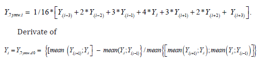
Pd data [based on proportional deviations from exponential trendlines between start (α) and end points (ω)], via their Pearson correlations, regressions and visual charts can give a new (?) method to evaluate similarity, especially simultaneousness in variation and possibly “pick up” some details, undetectable by linear regression analysis with native data. PS. The pd method/experiment is resembling an earlier “7ymw-experiment”, skizze, in [6]: Figure 5 presents derivative changes of (K/ Mg).fm and nCHD are got via their “7 year mean weighted means” (7ymw):
nCHD = non-CHD = Total mortality minus CHD. It worked in this Figure, but not in several materials. Possibly sometimes.
Synthesis and In Silico Analysis of Chalcone Derivatives as Potential Prostaglandin Synthetase Inhibitors
Summary
Prostaglandins (PGs) are biochemical endogenous lipids with autacoid functions, synthesized in- vivo from arachidonic acid [1]. PGs and other similar physiologically active compounds are collectively known as metabolites of eicosanoids [2]. PGs have long been reported to have sustained homeostatic roles and facilitate many pathogenic mechanisms in inflammation, gastrointestinal tract [1], muscle contraction, blood clotting [3], ocular protection [4,5], and regulation of the circulatory system [6,7]. These lipids are produced via the action of the cyclo-oxygenase (COX-1 and COX-2) isoenzymes, and their biosynthesis is antagonized by the nonsteroidal anti-inflammatory drugs (NSAIDs) [1]. Some vitamins, including D3 (cholecalciferol), and K2 (menaquinone) are also known to inhibit the actions and biosynthesis of PGs [8-10]. PGs mainly take part in vasodilation, conception, luteolysis, menstruation, parturition, blood pressure reduction, control of sodium reabsorption by the kidney, etc [11]. Studies have shown that excessive concentrations of PGs induce diarrhea that accompanies medullary carcinoma of the thyroid or neural crest tumors and mediates several inflammatory responses [11], incoordinate hyperactivity of the uterine muscle leading to uterine ischemia, and menstrual cramps in women [12]. PG structural analogs like latanoprost, travoprost, and bimatoprost with antagonistic properties, are being used and well-tolerated for the reduction of intraocular pressure (IOP) in patients with primary open-angle glaucoma and ocular hypertension [7].
Previous reports have indicated that there are some correlations between high levels of PGs analog (PGFS) in tumors of the GI tract and the effectiveness of NSAIDs [13]. Thus, they can be used in the study, design, and discovery of antitumor agents. Cyclooxygenase 1 and 2 (COX-1 and COX-2) biologically transform arachidonic acid (AA) to prostaglandins H2 (PGH2), which is further biotransformed to various PGs, and other endogenous lipids like thromboxanes, leukotrienes, and hydroxyeicosateraenoic acids [14,15]. The names of these enzymes are derived from their catalytic cyclo-oxygenation that converts AA to prostaglandin G2 (PGG2), and peroxidation of PGG2 to PGH2, hence are also known as peroxidase enzymes as well [16]. The three COX isoforms, COX-1 COX-2, and COX-3, have been identified to share almost 60% amino acid sequence similarity but with much higher sequence homology in the catalytic sites (Figure 1) [17]. COX-1 is firmly expressed in many tissues, while COX-2 is strongly induced by various mitogens and plays imperative roles in many pathological conditions like inflammation [18,19]. There is also a COX-3 enzyme but reported to be not functional in humans. COX-3 isozyme is encoded by the same gene as COX-1, but COX-3 retains a particular nucleotide sequence (intron 94) that is not retained in COX-1 [20].
Figure 1
PGE2 increases gastric mucus secretion, uterus contraction (particularly during pregnancy), GI tract smooth muscle contraction, inhibition of lipolysis, autonomic neurotransmitters regulation, platelet response to agonists, and in-vivo atherothrombosis [21,22]. COX-1 enzyme regulates the baseline levels of PGs, while COX-2 synthesizes PGs via stimulation and significantly increases PGs levels during growth and inflammation, although both enzymes are located in the stomach, kidneys, and blood vessels [23]. Hence, inhibition of these agents is necessary for the optimal regulation of many biological functions, when in excessive amounts. NSAIDs inhibit the activities of COX-1 and COX-2 enzymes. There are non-selective (inhibits both COX-1 and COX-2), and COX-2 selective NSAIDs. These NSAIDs, while reducing inflammation caused by PGs, also inhibit platelet aggregation and increase the risk of GIT ulcers and intestinal bleeding [24]. COX-2 selective inhibitors promote thrombosis and increase the risk of heart attacks [25]. Due to these adverse reactions, coupled with the high etiology of vascular, and kidney disease complications, some COX-2 inhibitors are no longer in clinical use [26]. There are also reports that NSAIDs impair the production of erythropoietin, resulting in anaemia [27].
The long-term harmful effects of most NSAIDs outweigh the medical benefits. A study conducted a few years ago, observed a statistically significant increase in myocardial infarction incidence among patients on rofecoxib [28], and data from approved clinical trials, showed a significant relative risk of cardiovascular events that led to the global withdrawal of rofecoxib in 2004 [29]. Another study reported a significant increase in erectile dysfunction in men who frequently used NSAIDs [30]. NSAIDs are also associated with a doubled risk of heart failure in people who have not experienced cardiac disease in their lifetime [31]. Finally, the use of NSAIDs during late pregnancy can cause miscarriage [32], premature birth [33], constriction, and closure of fetal ductus arteriosus, leading to different blood-related congenital heart diseases in the fetus [34]. Acetaminophen, regarded as the safest, and well tolerated NSAID during pregnancy, was reported to cause male infertility in the fetus [35,36]. These advents call for the search for more effective, with minimal toxic molecules that can be used clinically to alleviate inflammatory conditions.
Chalcones chemically known as 1,3-diaryl-2-propen-1-ones, are flavonoids and isoflavonoids precursors, are chemical moieties present in many naturally compounds and are also prepared synthetically because of their convenient synthetic procedures [37]. Chalcone derivatives have been reported to possess antiproliferative [38], anti- inflammatory [39], antitumor [40], antimalarial [41], antibacterial [42], antiviral [43], antileishmanial [44], antifungal [45] properties, among others [46]. Molecular docking is a veritable tool used in the computational prediction of ligands and protein inhibitory affinity in the search for lead molecules [47], including characterized natural products [48]. Therefore, we conducted the synthesis and molecular docking of some chalones derivatives which biological properties were evaluated previously, that can serve as lead compounds in the design of anti- inflammatory and analgesic agents, especially as potential prostaglandin synthetase enzymes (COX-1 and COX-2) secretagogues inhibitors.
Method
Synthesis
Scheme 1: Synthesis of Methoxy, Halogenated and Aminated Chalcone Derivatives: All reagents used in the synthesis and other analysis were of analytical grades. The IR data was obtained from the FTIR-8400S instrument, Shimadzu global links, North America, while Nuclear Magnetic Resonance (NMR) experiment was performed on a 400 MHz instrument, obtained from Varian Inc. Palo Alto, California, USA. An equivalent weight of 10.6 g benzaldehyde and 12.0 g acetophenone were weighed, into a 100 ml flask having 25 mL EtOH, and stirred on ice (4-0℃). 20 ml of KOH (20%) was added with continuous stirring for 20 minutes and allowed to stand for 24 hours. Ice chips were added, and the mixture was titrated with 25 mL of 20% acetic acid (4-0℃). Precipitates were formed, filtered under suction and recrystallized with ethanol, dried, the percentage yield and melting point were determined. This procedure was repeated with different benzaldehyde derivatives, including para-methoxybenzaldehyde, para-chlorobenzaldehyde and para-dimethylaminobenzaldehyde, giving rise to various derivatives of chalone (Scheme 1).
Scheme 1
Scheme 2: Synthesis of 6-Diphenyl-2-Thiopyrimidine Chalcone Derivatives: From the initial 4-methoxy-chalone derivative obtained, an equivalent weight of 2.38 g 4- methoxy-chalone, 2.12 g sodium bicarbonate, and 1.52 g thiourea, were weighed into a flask having 30 mL DMSO. The mixture was refluxed under Nitrogen gas for about 2 hrs, using a Thin Layer Chromatographic plate to monitor the progress of the reaction. Water was added to the reaction medium at the end and was allowed to stand for 24 hours. Precipitates were formed, filtered under suction, the residues were recrystallized with diethyl-ether and petroleum spirit. The percentage yield and melting points of the crystals obtained were quantified, after drying (Scheme 2).
Scheme 2
Scheme 3: Synthesis of Epoxide Chalcone Derivatives: For the synthesis of epoxide derivatives, an equivalent weight of 5.16 g chalcone obtained previously was weighed into a beaker; 10 ml of 10% NaOH and 60 ml of MeOH were added respectively. The content of the beaker was dissolved with stirring via gentle heat, then 20 ml hydrogen peroxide H2O2) was added and stirred for 30 minutes. 5 ml of 10% acetic acid was used to acidify the medium. The resultant product was collected, and recrystallized with MeOH, filtered and dried. The percentage yield and melting points were respectively determined. This procedure was repeated with para-methoxychalcone, para-chlorochalcone, para- dimethylaminochalone, respectively, leading to the production of chalcone epoxide derivatives (Scheme 3).
Scheme 3
Molecular Docking
Molecular modeling and docking simulations of the binding protein and synthesized ligands were done using the Maestro software of OPLS3, 2018 Force field [49], and Pymol software [50]. The docking parameters and affinity were compared with the previously reported pharmacological profile of the chalcone derivatives. The human COX-1 crystal structure protein (6Y3C) [51], and 1PXX (COX- 2 crystal structure with diclofenac bound to the cyclooxygenase active site) [52], were obtained from the PDB website, and modeled with the Pymol and D3Pocket webserver [53,54], to obtain all possible binding pockets and utilize one(s) with the highest affinity using diclofenac and Celecoxib (a selective COX-2 inhibitor) as the standard molecules.
A. (E)-Chalcone. B. Para-chlorochalcone [(E)-3-(4-chlorophenyl)-1-phenylprop- 2-en-1-one] C. Para-methoxychalcone [(E)-3-(4-methoxyphenyl)-1-phenylprop- 2-en-1-one] D. Para-dimethylaminochalcone [(E)-3-(4-(dimethylamino) phenyl)-1-phenylprop-2-en-1-one] E. Para-methoxy-4,6-diphenyl-2-thiopyrimidine[4-(4-methoxyphenyl)- 6-phenyl-5,6 dihydropyrimidine 2(1H)-thione] F. Chalcone-epoxide [phenyl(3-phenyloxiran-2-yl) methadone] G. Para-chlorochalcone-epoxide [(3-(4-chlorophenyl) oxiran- 2-yl) (phenyl)methanone] H. Para-methoxychalcone-epoxide [(3-(4-methoxyphenyl) oxiran- 2-yl) (phenyl)methanone] I. Para-dimethylaminochalcone-epoxide[(3-(4-(dimethylamino) phenyl)oxiran-2-yl)(phenyl)methanone]
Discussion
The compounds were obtained in high yield after the synthetic processes (Schemes 1 & 2). The percentage yields of the compound ranged from 27.68 – 90.38%, with sample B having the highest yield while sample I gave lowest synthetic yield. Also, the spectroscopic (FTIR and NMR) analysis shows distinct spectrum across all molecules, indicating the presence of unique functional groups and chemical environments (Table 1). All the synthesized chalcones derivatives showed appreciable protein binding affinity against the COX-1 and COX-2 enzymes. Compared to the standard drugs, better protein-ligand affinity was observed with COX-2 enzyme. Diclofenac is known to inhibit both COX-1 and COX-2 enzymes [55]. The computational experiment showed that, some of the synthesized compounds had higher binding affinity against the COX-1 protein than both diclofenac and celecoxib. Compound A showed the highest affinity (-7.24 kcal/mol), while other compounds had affinity level of -7.21(C), -7.16 (B), -7.14 (I), -7.10 (D), -7.00 (H), -6.92 (G), -6.88 (F), and -6.11 kcal/mol(E), respectively. Whereas, the standard compounds (diclofenac and celecoxib) had -5.46 and -6.19 kcal/mol, respectively.
Table 1: Physiochemical and elemental analysis of Chalcone derivatives.
The protein-ligand interactions showed the actual protein residues in the COX-1 protein that compounds bound with (Figure 2). Also, the binding pocket and pose of the compound with highest affinity showed how it is well fitted into the protein pocket (Figure 3). Celecoxib, a selective COX-2 inhibitor showed highest binding affinity of -10.55 kcal/mol, while the test compounds had -8.55 (A), -8.84 (B) -8.50 (C), -8.79 (D), -8.24 (E) -8.13 (F), -8.50 (G), -8.22 (H), -8.69 (I), and diclofenac had -8.49 kcal/mol respectively (Table 2). The binding interactions of all molecules are shown in Figure 4, while binding poses of the molecules with the highest affinity is illustrated in Figure 5. Compounds E (4-methoxy-4,6-diphenyl-2-thiopyrimidine) and B (para-chlorochalcone) from previous studies, displayed remarkable anti-inflammatory in an in-vivo analysis using animal model [39]. E also showed the appreciable affinity against COX-1 protein more than the standard compounds, while lower affinity was observed against COX-2 protein. For compound B, it showed the highest affinity against COX-2 and very high affinity towards COX-1 protein compared to the standard molecules used in the analysis. This shows that with adequate physiochemical and structural modifications, these compounds could serve as potential lead compounds in analgesic and anti-inflammatory pharmacology, as pain and inflammation are associated with these enzymes in the biological system [16].
Figure 2
Figure 3
Figure 4
Figure 5
Table 2: Structural features and Molecular docking of the synthesized compounds.
Conclusion
Analgesic and anti-inflammatory agents are used in the prevention of all kinds of pains, ranging from minor headaches to severe post-operative pains. The search for newer agents due to poor tolerability, adverse reactions and affordability of the existing ones is the focus of contemporary drug design and development. The compounds showed highly promising results in both in-vivo and computational molecular docking studies. Hence, the compounds reported in this study could be utilized and further modified structurally and physiochemically to achieve better analgesic and anti-inflammatory properties.
Impact of Die Configuration on Physio-Chemical Properties, Anti-Nutritional Compounds, and Sensory Evaluation of Multi-Based Extruded Puffs
Introduction
Millets are highly valued by vegetarians, vegans, and individuals with coeliac disease for their exceptional nutritional benefits [1]. These plant-based foods are abundant in proteins and complex carbohydrates while being low in fat [2]. Additionally, they are a rich source of dietary fiber, essential minerals, and B-group vitamins [3,4]. However, Millet preparation can be a time-consuming process as they require prolonged soaking and cooking, which reduces their consumption by consumers [5]. To overcome this challenge, novel food products like – ready-to-eat Millet-based snacks could be developed. Such products could encourage more individuals to incorporate Millet into their diet [6]. The food processing technique of extrusion- cooking is highly versatile, multifunctional, and cost-effective. Raw materials are exposed to heat, pressure and shear forces during this process, leading to various biochemical reactions such as protein denaturation, starch gelatinization, fiber degradation, amylose-lipid complex formation through Maillard reaction [7]. Extrusion-cooking is commonly employed to create expanded snacks that are ready-toeat, come in different shapes and textures, and boast enhanced flavour and colour [8]. High concentrations of raffinose-family oligosaccharides (RFOs) in lentils cause stomach discomfort and reduce lentil quality for human consumption.
To develop strategies for lentil quality improvement, variability, heritability and effects of environmental conditions on the content and composition of soluble carbohydrates in lentil seeds have been investigated in detail [9]. Over the past few years, there has been significant research on creating extruded products using Millets [10]. In most cases, these Millets are blended with wheat [11]. Numerous studies have examined the impact of various extrusion-cooking factors, including feed moisture, screw speed, extrusion temperature, nutritional characteristics [12] physico-chemical, sensory and textural properties of prepared product. These studies have also included trials conducted directly at the industrial level [13,14]. However, there has been a lack of research on how the die configuration, which determines the final product’s shape and size, affects the extrusion of Millets. Food shape and size play a critical role in capturing the consumer’s attention [15]. These features strongly influence the implicit associations with consumers concerning nutritional value [16]. Moreover, the shape and size of food can significantly impact the sensory qualities and physico-chemical properties of the extruded product [17]. Therefore, the present study was designed to examine the impact of star shaped and circular die configurations, which have two different diameters of 35.9 and19.6 mm², respectively, on the anti-nutritional component, physico-chemical properties, and sensory features of extruded snacks made from Millet flour.
Materials and Method
For the development of extruded puff products, germinated pearl Millet (Pennisetum glaucum), finger Millet (Eleusine coracana), sorghum (Sorghum bicolour), foxtail Millet (Setaria italic) and rice (Oryza sativa) as base were used as raw materials for the present study work. These Millets were procured from a nearby local market in Meerut, Uttar Pradesh [18].
Optimization of Single Screw Extruder Operating Parameters for Different Millet Based Extruded Puffs Products
The operating parameters of the twin screw extruder mainly, the temperature, feed moisture content and the screw speed, were optimized for the various “best selected” four Millet fortified with rice based extruded puff products formulation. Three feed moisture content (20%, 25%, and 30% wt.b.), screw speeds (180, 270, and 360 rpm) and 160, 180°C and 270°C temperature were selected to produce extrudes. The extruded samples were then analyzed for physical analysis like expansion ratio, water holding capacity, moisture content, puffing properties and texture analysis. Further experiment was carried out at three different level of temperature (100, 110 and 120°C) with keeping constant screw speed and feed moisture content.
Sample Preparation from Extrusion
Laboratory scale single-screw extruder (Model no: GTL-100), (Zigmo Agro Pvt. Ltd. New Delhi, India) was used for sample preparation. During each extruder run, the extruder machine was allowed to equilibrate for 5-10 min until a stable torque was achieved. Extruded samples were collected on metal screens to allow excess steam to flash off. The extruded samples were collected in a low-density polyethylene bag after cooling and stored in a cool and dried area.
Development of Extruded Puff Products Based on the Millet’s Combinations
Extruded puffs preparation was done, and it mainly consists of puffs mixture of Millets in combination as shown in Tables 1 & 2 and rice is used as base. The blended puffs mixes at appropriate moisture content were extruded to produce extruded puff through the extrusion machine (manufacture: Jas Enterprises, Ahmadabad, India) into desired shaped products and developing extruded puff products based on Millet combinations involves a series of steps to create a desirable texture, flavor, and nutritional profile the process flow chart shown in Figure 1.
Figure 1
Multi Millet Conditioning
To achieve the optimal moisture concentration for extrusion (16 g/100 g), the Puffs were conditioned. The amount of water required to reach this moisture level was determined based on the initial moisture content of each flour type, which was 12.95 ± 0.01, 10.87 ± 0.01, and 12.54 ± 0.06 for pearl Millet, finger Millet and foxtail Millet, respectively. Water was added gradually to the flour in dough mixer at average speed to avoid the lumps formation. The process took approximately 20 minutes to obtain uniformly hydrated flour.
Extrusion-Cooking Process
Extrusion cooking is a food processing technology that integrates multiple operations such as mixing, cooking, kneading, shearing, shaping, and forming [19]. The DSE30 Lab Twin-screw extruder was used to carry out the extrusion-cooking process with a 12 kg/h capacity. The extruder machine design had two 38CrMoAl screws, a 5-kW motor and operating at maximum screw speed of 500 rpm, with three heating zones at 55, 95, and 125°C, respectively. The extrusion process was carried out using circular and star-shaped dies holes with cross-sections of 19.6 mm2 and 35.9 mm2, respectively. The circular die nozzle and star cross-section had a length of 6.35 mm. The feed rate was set to 2.5 g/s, the die temperature to 160°C, and the screw speed to 230 rpm. To examine the extruded products, the water absorption index, water solubility index, starch gelatinization degree, colour, phytate and oligosaccharides content were measured. For this purpose, extrudates were ground using an electrical grinder (HM- 5735) from Home Electrical Appliance and passed through a 0.25 mm sieve sized blades for some analysis, while other analyses were performed on the entire extrudates.
Physical Assessment of Extruded Puff
Finger Millet (Eleusine coracana L.), pearl Millet (Pennisetum glaucum), foxtail Millet (Setaria italic) and sorghum (Sorghum bicolour) are three selected cereals that have been evaluated in terms of physical parameters, specifically bulk density, in the context of cereals and cereal-based products. The evaluation of bulk density for the three combinations of puff products made from the selected cereals would involve measuring the mass and volume of the cereal products. The mass can be measured using a scale, while the volume can be determined by various methods such as displacement or geometric calculations. By studying and analysing the obtained results of bulk density, these conclusions can help in understanding the texture, density, and overall quality of the products, which are important factors for consumer acceptance. It’s worth noting that in addition to physical parameters like bulk density, other nutritional and sensory attributes of these cereals and their products are also crucial for evaluating their overall nutritional value and consumer appeal [20]. These may include factors such as nutrient composition, digestibility, taste, aroma, and shelf life, among others. By conducting such evaluations, can gain insights into the potential of these cereals and their products as staple foods and nutrient sources, both in developed and developing countries. Kjeldahl digestion methods (Advanced and ordinary) compared total nitrogen in non-germinated and germinated extruded puff products. Advanced Kjeldahl showed protein variations of (07.11% to 10.66%) and (09.45% to 11.98%), while ordinary Kjeldahl showed (05.11% to 10.96%) and (07.45% to 11.56%). Millet combinations revealed T3 with germinated Millets had higher protein, indicating nutritional value. Total ash, dietary fiber, and carbohydrates varied in extruded puff products. Statistical analysis indicated significant differences (p<0.0001) for each combination. Incorporating Millet and sorghum in rice flour (T3) resulted in higher protein and overall acceptable sensory properties. AOAC methods revealed significant differences (p=0.05) in proximate compositions of multi-Millet puffs with overall acceptable sensory properties [20]. This knowledge can be valuable for food scientists, policymakers, and nutritionists in promoting sustainable and nutritious food options worldwide.
Bulk Density and Expansion Ratio
Extruded products bulk density (BD) was studied by using the rapeseed displacement method and calibrated as per given equation (1) by [21]. For this purpose, the (10 ± 0.1 g) of randomly selected extruded product were weighted:
Whereas Wt. and Vep-1 are the weight in (gm) and the equivalent volume (cm3) of the extruded products, respectively. Actually, Vep is multiplication ratio between the rapeseed density (ρs) and the rapeseed weight (Ws), with same volume as the extrudates. Five replicates for each sample were prepared to study the parameters. sectional expansion index (SEI), bulk density (BD), instrumental color, and dry and bowl-life texture were evaluated. SEI and BD responses were fixed by moisture variable is incorporated; darker products were produced. Nevertheless, high together with higher temperature and lower moisture levels produces better color appearance. At high ratio desirable low hardness and crispy expanded extrudates can be generated as long as moisture is lower than about 22% [22]. The calibration of expansion ratio (ER) was according to the ratio of extruded product diameter to determine the die hole diameter of extruder with the help of caliper device, as reported by Kokseland Masatcioglu. For this purpose, ten replicates were taken for (ER) assessment.
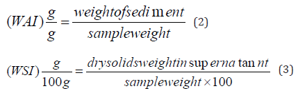
Water Absorption Activity
The extruded products water absorption index (WAI) and the water solubility index (WSI) were determined as per equations (2) and (3) [23].
The (WSI) is the dry solid weight in the extracted supernatant, whereas (WAI) is the sediment weight without the supernatant per unit weight of the sample analyzed. Each sample was tested in a triplicate manner.
Starch Gelatinization
The starch gelatinization (SG) of the extruded products determination follows the modified method based on the procedure outlined by [24]. This method involves the formation of a blue iodine complex when amylase is released during gelatinization. Specifically, 40 mg quantity of sample was dissolved in a 50 mL of 0.15 M KOH solution and mixed thoroughly for 15 minutes. The reaction mixture was then centrifuged at 4032 x g for 10 minutes to remove out insoluble sediment. Next, 1 mL quantity of the supernatant was neutralized by the addition of 9 mL of 0.017 M HCl, and 0.1 mL of iodine reagent (1 g iodine and 4 g potassium iodine dissolved in 100 mL water). The resultant solution was mixed, and read the absorbance at 600 nm (A1) using a Cary 60 UV-VIS spectrophotometer. In addition, 1 M KOH and 0.1 M HCl solution was used to prepare control samples. The overall value of DG was calibrated by using equation (4) based on the average of three replicates.
Whereas (A1/A2) is the ratio of absorbance at 600nm of the sample to that of the control.
Phyto-Chemical Constituents of Selected Millets Puffs
The effect of extrusion processing on anti-nutrients factors namely tannin, phytate and saponin of extruded Millet-sorghum blend rice puffs puff product combinations were studied. Extrusion processing is necessary to absorb essential micro and macronutrients from added blends of puffs during extruded snacks preparations and eliminates a negative effect of anti-nutritional factors such as tannin, phytate and saponins. Thus, nutritional quality was maintained by extrusion through destruction of anti-nutritional components.
Color Determination
The CM-600d colorimeter (Konica Minolta Sensing Inc., Osaka, Japan) was used to determine the lightness (L*), redness (a*), and yellowness (b*) of both Puffs and extruded products with help of using the Spectra-Magic NX software (Konica Minolta, Tokyo, Japan). The series of experiments was replicated five times in a row.
Oligosaccharides Analysis
The presence of oligosaccharides namely verbascose, stachyose, and raffinose in Puffs and extruded products were investigated by using the HPLC with slight modifications in a method prescribed by [25]. Samples were mixed with deionized water, filtered, and separated isostatically on a cation exchange column. Identification was based on standard comparison, and quantification was based on calibration curves. Results are expressed in (mg/g dry matter) of each oligosaccharide after triplicate analysis.
Phytate Analysis
The phytate content of both Puffs and extruded products was determined by following the [26] method as its values were expressed in (mg/g) of dry matter of phytic acid. To calculate the phytate content, obtained values were multiplied by 0.282 and it is the molar ratio of phytate-phosphorus in a molecule of phytate. The analysis was done in a triplicate manner.
Sensory Evaluation
A panel of 28 semi-trained judges from University of Life Sciences and Technologies demonstrate Millet-based extruded snacks using a ranking test. Each sample is arranged in groups of three on glass plates to evaluate appearance, texture, taste, and aftertaste using an evaluation form as this form is generated through Fizz Acquisition 2.51 software. Warm black tea was used for taste neutralization between samples. The panelists ranked the samples as per most liked=1 to least liked=8 and the recorded results were calibrated as the summation of ranks for each sample (Figure 2).
Figure 2
Statistical Analysis
The recorded data of Millet Puffs and extruded products undergo one-way ANOVA and two-way ANOVA stats analysis, followed by Tukey’s HSD test. The two-way ANOVA stats analysis considers two major factors namely Millet puffs type and die type for further analysis. Minitab-17 ver. statistical software (Minitab, Inc., State College, PA, USA, 2010) was used to determine the significant differences among all studied parameter values at p < 0.05. The sensory evaluation data were statistically analysed by using the Friedman test with Fizz calculation (Biosystems, Cousteron, France) and a p<0.05 level of significance.
Results and Discussion
The various multi-Millet utilized to produce extruded snacks were shown in Table 1. Table 1 showed the notable differences among (L*, a*, and b*) colour patterns. Pearl Millet flour exhibited the highest a* and b* values while it had lowest L* value. In contrast, foxtail Millet flour had lightest colour, followed by finger Millet flour. Foxtail Millet flour exhibited the lowest a* and b* values, with the latter being statistically insignificant in comparison to pearl Millet flour. Additionally, Table 2 calibrated values were significantly differed (p<0.05) as the amount of anti-nutritional compounds were studied among the Puffs. Millets are known to contain several anti-nutritional compounds, including non-digestible oligosaccharides and phytic acid, which has inherent chelating characteristics to capture important divalent cations such as Fe, Zn, Ca, and Mg, which leads to lowering of availability for absorption and use in the small intestine [27,28]. However, presence of raffinose, verbascose, and stachyose oligosaccharides in human diets in an ample amount causes flatulence and discomfort in humans after consumption [29,30].
Table 1: Color parameters of Millet flour of pearl Millet, finger Millet and foxtail Millets.
Note: *Each (n = 3) replica values were expressed as (mean ±standard deviation).
Table 2: Physicochemical parameters of spherical and star-shaped extruded products obtained from different Millets Puffs.
Note: *Each parameters value was expressed as (mean ± standard deviation) for (n=3).
Pearl Millet flour exhibited the highest concentration of phytates, followed by finger and foxtail Millets Puffs, respectively. Foxtail Millet flour contained the highest levels of verbascose, although it had stachyose in a lesser amount. Similarly, finger Millet flour had the highest amount of stachyose, while it has lowest amount of raffinose. However, the quantity of oligosaccharides in Millets varied as per the selected species and varieties, as well as the existing environmental conditions [31,32]. [33] reported significant variability in the amount of raffinose (4.10–10.30 mg/g), stachyose (10.70–26.7 mg/g) and verbascose (0.00–26.70 mg/g) among 18 different pea varieties. While Tahir et al. (2011) observed higher stachyose levels than raffinose and verbascose in 11 lentil varieties, as these findings were found in line with current findings. This difference in oligosaccharides level might be due to significant constraint on the extensive use of legumes at both domestic and industrial scale [34] (Figure 3).
Figure 3
Physico-Chemical Properties of Extruded Products
All physico-chemical parameters had significant differences (p < 0.05) among the extruded products, except water absorption index (WAI). These noticeable differences were attributed due to the type of Millet used, the type of die, and the (Millet x die) interaction, as shown in Table 3. However, it should be noted that the type of die had no significant effect on the WAI. Pearl Millet-based extruded products had the highest bulk density (BD) and water absorption index (WAI), whereas it has lowest expansion ratio (ER) and water solubility index (WSI) values. Similarly in foxtail Millet-based products had the highest (ER) and well-expanded spherical extrudates, while highest degree of starch gelatinization (SG) was recorded in finger Millet-based products. Higher ER, DG and WSI with lower BD was recorded in circular die configuration based extruded products as compared to star-shaped die. The effect of die shape on extruded product characteristics can be explained by change in friction and pressure strength. The circular die had a smaller cross-section, resulting in higher levels of friction and pressure and thus higher temperatures, which led to more expansion and lesser dense products, will obtain as it has greater ER and lower BD. On the other hand, the star-shaped cross-section had angles that could have mechanically broken bubbles in the gelatinized starchy matrix, which led to disturbance in expansion. However, with increment in the die nozzle diameter decreased radial expansion in yellow corn extrudates. Along with this, inducing higher extrusion pressure on starch gelatinization causes expansion of the extrudates products made from foxtail and finger except in pearl Millet-based products since it has higher fibre content that restricted starch gelatinization [1], [35]. Although ER and BD are important physical parameters that can influence consumer behavior in the sense of acceptability of extruded products [36].
Table 3: Color parameters of spherical and star-shaped extruded products obtained from different Millet Puffs.
Note: *Each parameters value was expressed as (mean±standard deviation) for (n=3).
Earlier studies by [37] who reported an inverse relation between BD and ER, as observed in this work, where a negative correlation was found (r = -0.631; p = 0.093). The presence of huge number of fibres in the feed Puffs can also affect the ER and BD values by reducing overall expansion on account of cell-wall rupture, resulting in a compact and hard product with an undesirable texture. In this context, Red lentil flour, with the highest fibre content, led to extrudates with the lowest ER and highest BD indicating the importance of considering fibre content while developing extruded product as described by [38]. The extrusion-cooking conditions, including the die used, may also impact the WAI and WSI values, which represent the amount of water that can be absorbed by the extruded product and the quantity of soluble substances formed during the extrusion process from starch, proteins, and fibres. The presence of fibres in higher amount could also influence functional properties [39]. Instead of this, WSI was also influenced by other factors such as legume type, die shape, and legume-die interaction, while effect of die shape had no significant effect on WAI. Higher fibre levels in the legume led to an increase in WAI, as they absorbed and retained water within a well-developed starch-protein-polysaccharide network, as discussed previously by [40].
Extruded Products Color
Colour is a crucial aspect of food products that can significantly affect consumer acceptability. Extrusion-cooking affects the colour features of the products, making them darker than the Puffs. The colour components of the extrudates were influenced by Millet type, die configuration and their interaction. The observed colour features were attributed to existing pigments and the Maillard reaction occurring during extrusion-cooking (Table 4). Star-shaped extrudates had greater L* and lower a* values (except for pearl Millet) compared to spherical shape extrudates, while b* index had found non-uniform trend. This fluctuating trend is due to pigment degradation as temperature rises and shear stress during extrusion is responsible to alter color, especially for carotenoids. The decrement in L* and increment in a* values may be linked to the melanoidins formation during the Maillard reaction, while increment in b* may be results from the formation of yellowish compounds during the initial stages of the Maillard reaction or from lipid oxidation. An advantage of larger die cross-section reduces extrusion pressure and heat, leading to a less intense Maillard reaction and reduces browning and flavor development [41]. Thus, star-shaped extrudates were obtained with the help of larger cross-sectional die and a less drastic extrusion process involved to obtain lighter colour than spherical shaped extrudates [42].
Table 4: Anti-nutritional compounds of spherical and star-shaped extruded products obtained from different legume Puffs.
Note: *Each parameters values were expressed as (mean± standard deviation; n = 3); indicating the significant differences (p < 0.05) among the sphere and star shaped products considering the interaction between the Millet and die.
Anti-Nutritional Component of Puffs and Extruded Products
The extrusion-cooking process and the type of raw material used can influence the levels of anti-nutritional compounds in legume extrudates [43,31]. A comparison of the native Puffs shown in Table 2 and the extrudates in Table 4 revealed different kind of behaviour for various anti-nutritional compounds. In present study the phytates content decreased as the extrusion-cooking of finger Millet (12% on average) and foxtail Millet (7.9% on average) Puffs initiated for both star-shaped and spherical products, possibly on account of thermal processing that is associated with the extrusion-cooking process. [12] found that total phytates were more greatly reduced in lentil flour extruded at 160°C compared to 140°C. However, oligosaccharides, particularly stachyose and raffinose increased during extrusion cooking. This could be attributed to the high temperature and pressure involved in extrusion-cooking, which break the bonding between oligosaccharides and other macromolecules, or alter the food matrix structure, leading to better extractability of anti-nutritional compounds [6]. Similar kind of results were observed in pea-rice gluten-free expanded products and extruded lentil snacks by other researchers [6,25]. It was observed that there were differences in verbascose, stachyose and raffinose content in Millets extrudates just because of Millet type, die configuration and their interaction, but their phytic acid was not affected by die shape. In case of pearl Millet based spherical extrudates have higher verbascose content than starshaped, while raffinose content increased to 7% in the latter. Common bean-based star extrudates had higher stachyose and raffinose content compared to spheres made from the same flour, which decreased by 1.7% and 7.5%, respectively [23]. Extrusion conditions and legume type affected oligosaccharide behaviour, with a higher temperature and pressure increasing stachyose and raffinose contents. An obtained results showed that oligosaccharides content was found higher in spherical shaped products than the star-shaped after die inducing higher pressure and heat generation, particularly for raffinose [39].
Sensory Evaluation of the Extruded Products
The sensory attributes like appearance, texture, taste, and aftertaste of the extruded products were significantly (p <0.05) affected by the type of flour and die used. The products ranking is decided as per test results (Table 5). As per sensory attributes the star-shaped extrudates prepared from pearl Millet were found to be least preferred acquiring lowest rank sum for “texture” due to their hard structure and difficult to chew, bland taste, and aftertaste. However, pearl Millet based spherical extrudates were liked for “appearance” and “aftertaste”, similarly notified in spherical and star-shaped extrudates from finger and foxtail Millets. Previously [10] studies showed that high values of BD and hardness can produce undesirable products for consumers. In contrast, common Millet extrudates, particularly a spherical one, were preferred in terms of all considered attributes owing to their properly puffed and crunchy nature, pleasant taste and aftertaste as discussed by [28]. In another study, extrudates made from blends of red lentil and corn were found to be more accepted than including (100%) lentil extrudates [17]. In general, the spherical shaped extruded products were favored as compared to star-shaped ones, indicating that preferred shape plays a crucial role in consumer perception and acceptability of food products. This is supported by studies that suggest that shape can even affect taste perception. However, there was no significant difference observed between spherical and star-shaped extrudates in terms of taste and aftertaste, possibly because textural features, such as appearance and structure, had a greater impact.
Table 5: Sensory characteristics of extruded (spheres and stars) shaped products.
Note: *Each parameters values were expressed as (mean± standard deviation; n = 3).
Conclusion
The study aimed to understand how the die configuration affects the extrusion of Millets. Most industry dies have a circular cross section, but the effect of a star-shaped die on Millet was still unknown. Obtain results of the study showed that the die-hole diameter significantly affects the physicochemical properties and sensory qualities of the extruded snacks. The use of a star-shaped die to produce products with a lower ER and higher BD than spherical extrudates and it is preferred one on account of lowering the friction resistance during extrusion. The increased knowledge on die configuration could aid in the expansion of Millet-based raw materials at maximal level to meet consumer satisfaction for healthy and palatable food products.
Nigella Sativa use for the Treatment of Cancer Tasawar
Introduction
Cancer is a big problem in society today and is the second most common cause of death after heart attacks. Every year, many people die from different types of cancer, even though we try really hard to find ways to stop and treat it. In the last 100 years, modern medicine has made big progress in treating diseases. But a lot of illnesses, like different types of cancer, are still not completely treated. Researchers are looking at both old and new ways of healing to find new and effective treatments [1]. Nigella sativa has been used as medicine for a long time. This tradition started in Southeast Asia and then was used in ancient Egypt, Greece, the Middle East, and Africa. The Islamic tradition and the healing power of medicine are important for healing and are an unusual type of medical treatment [2]. This plant is a flower plant and its seeds are used as a spice in cooking. In English, the seed is often called black cumin, and in ancient Latin it was named “Panacea”, showing that it was used for healing. In Arabic, the seed is called “Habbah Sawda” or “Habbat el Baraka”, which means “Seed of blessing”. In Arabic, people call the seed “Habbah Sawda” or “Habbat el Baraka”, which means “Seed of blessing”. This tree is called “Kalo jeera” in Bangladesh, “Kalonji” in India, and “Hak Jung Chou” in China [3]. The plant’s seeds and oils are important for medicine. The main parts of N. Sativa could help keep you healthy and might treat different illnesses like cancer. One way it works well is by lowering the chance of atherosclerosis. It does this by lowering bad cholesterol in the blood and raising good cholesterol. It helps diabetes by making the body healthier and protecting the cells that make insulin in the pancreas. This can help as a treatment for diabetes. Take care of and keep safe. It helps control high blood pressure [4]. It effectively reduces airway inflammation in people with asthma, and its components show potential as a complementary treatment for schistosomiasis. In addition, its oil also protects kidney tissues from damage caused by harmful oxygen molecules, thereby preventing kidney dysfunction and structural abnormalities. For countless centuries, seeds, oils and extracts derived from N. sativa have been used for their anti-cancer properties in traditional systems of medicine such as Unani, Ayurveda and ancient Chinese medicine. These systems were developed in Arabic, Indo-Bangla and Chinese respectively [5].
Role of sativa as Anti-Cancer Mediators
A lot of useful substances have been found in the seeds of N. Sativa is a type of cannabis plant. Instead, it should be written in a simpler and easier to understand language. Nsativa seeds contain oils, proteins, alkaloids and saponins. These components were analyzed to quantify four important pharmacological elements in the oil: thymoquinone, dithymoquinone, thymohydroquinone and thymol. Nsativa seeds are seeds of the sativa plant. The main component in the essential and fixed oils of the seeds, called thymoquinone, is believed to be responsible for a significant portion of their biological effects. Thymoquinone is often recognized for its powerful abilities as an antioxidant, anticancer, and antimutagenic agent. In addition, thymoquinone has acceptable safety levels, especially when administered orally to animals in experiments. Alpha-hederin is a compound found in black seed that comes from the seeds of the N. sativa plant [6].
Blood Cancer
Thymoquinone stops the growth of a type of cancer cells called HL-60 cells, which are found in human myeloid leukemia. Researchers studied different forms of thymoquinone with 6-alkyl residues and terpenes in HL-60 cells and 518A2 melanoma. The scientists discovered that these substances can cause a process called apoptosis, which is when the DNA breaks into pieces, the energy in the cell decreases, and there is a small increase in harmful chemicals. They found that α-hederin made P388 murine leukemia cells die by causing more apoptosis to happen, and this happened more as the dose of α-hederin and the time went up [7].
Breast Cancer
The mix of alfalfa, melatonin and retinoic acid helped lessen the bad effects of DMBA on breast cancer in mice. Thymoquinone was tried on breast cancer cells called MCF-7/Topo. Thymoquinone has a special part called terpene and 6-alkyl. They discovered that these substances made cells die through a process called apoptosis [7].
Colon Cancer
Thymoquinone can help fight colon cancer cells and promote cell death. This was shown in a study where the N.sativa volatile oil was used on colon cancer cell line HCT116. N.sativa can stop the growth of colon cancer in rats, after it has started, without causing any noticeable negative effects. Thymoquinone is a substance that can be used as a treatment for colon cancer cells. It works similarly to a drug called 5-flurouracil. However, thymoquinone did not have any effect on HT-29 (colon adenocarcinoma) cells [1].
Pancreatic Cancer
Thymoquinone is the most important chemical in Nigella sativa, which is known for its important healing properties. The study looked at sativa oil extract affects the way pancreatic cancer cells grow and die. Scientists have suggested using thymoquinone to stop inflammation and encourage cells to die in a certain way [8]. This could be a new way to treat inflammation. Thymoquinone can help make pancreatic tumors more sensitive to standard treatments by reducing the effects of gemcitabine or oxaliplatin on NF-kappa B activation. Mucin 4, a big molecule with sugar attached to it, is not working properly in pancreatic cancer. This strange expression is important for many things like cells change, grow, spread, and resist chemotherapy in pancreatic cancer. The study looked at thymoquinone affects MUC4 expression in pancreatic cancer cells [7].
Hepatic Cancer
A lot of research has been done to study well different treatments can kill cancer cells. This study wanted to see if sativa seeds can affect liver cancer cells grow. The test showed that N can stop HepG2 cells by 88% after being left with them for 24 hours at different amounts. So, using sativa extract is very important in academic discussions. Thymoquinone has been found to help the body’s quinone reductase and glutathione transferase work better when taken by mouth. The properties of thymoquinone make it possible to prevent cancer caused by chemicals and protect the liver from damage [9].
Lung Cancer
The cancer-fighting ability of α-hederin found in N.staiva is being studied. The research looks at sativa affects lung cancer in mice. A study also showed that putting honey and N. Adding sativa to the diet makes a big difference. Sativa helps protect against oxidative stress and inflammation caused by certain chemicals and can help prevent lung, skin, and colon cancer. Alfalfa has been looked at a lot because it might have healing powers [2]. These chemicals have different effects on living things, such as reducing inflammation, fighting cancer, and preventing damage caused by harmful substances. Additionally, they look like they could help treat heart problems and might assist in cancer treatment. Understanding α-hederin and thymoquinone work can help us use them in medicine. More research is needed to understand they can help people and make sure they are safe and work well in medical treatment. N sativa does not have a big impact on cell death or programmed cell death in lung and laryngeal cancer cells [10].
Skin Cancer
Topical use of N. sativa is a common form of management used in a variety of settings. sativa extract showed an inhibitory effect on the initiation and promotion stages of skin carcinogenesis in mice when administered intraperitoneally. Skin application of 20-methylcholanthrene resulted in a significant reduction in soft tissue sarcomas, which was limited to 33. 3%, compared to 100% incidence observed in the MCA control group [11].
Fibrosarcoma
Thymoquinone, taken from the seeds of Nigella sativa, has been studied a lot for its possible healing powers because of its different biological effects. The administration of sativa one week prior to and following MCA treatment exhibited a notable hindrance in the development of fibrosarcoma tumor occurrences, as well as a reduction in tumor mass, by 43% and 34% respectively, in comparison to the outcomes observed in the MCA solitary treatment group. Furthermore, it was observed that thymoquinone exhibited a delayed onset of fibrosarcoma tumors induced by the administration of MCA. Moreover, in vitro investigations demonstrated that thymoquinone exhibited inhibitory effects on the viability of fibrosarcoma cells. Alfalfa oil is a special kind of oil from the Medicago plant that can decrease the ability of human fibrosarcoma cells to break down fibrin in lab tests [1].
Renal Cancer
There is an existing body of research that highlights the potential chemo-preventive efficacy of N.sativa, a substance that has garnered significant scientific interest. N sativa has inhibitory effects on renal oxidative stress, hyperproliferative response, and iron nitrilotriacetate-induced renal carcinogenesis. In this experimental study, alfalfa was administered orally to rats for therapeutic purposes.The administration of sativa elicited a pronounced reduction in the generation of H2O2, synthesis of DNA, and occurrence of tumors [12].
Prostate Cancer
Thymoquinone comes from Nigella seeds and has many important medical qualities. The extract from the sativa plant can slow down the making of DNA, stop cells from growing, and reduce the ability of cancer cells in the prostate to survive. These changes were seen only in cells that have cancer, not in cells that do not have cancer. It was found that this result happened because the androgen receptor and transcription factor were decreased [13]. Thymoquinone was found to work well in treating both hormone sensitive and hormone-refractory prostate cancer in different experiments. Research done in the lab and in animals shows that thymoquinone can stop the growth of new blood vessels. In addition, thymoquinone was found to stop the growth of blood vessels in a human prostate cancer model in mice. Also, when used in small amounts, thymoquinone stops the growth of human prostate tumors, with very few chemical side effects. Furthermore, thymoquinone affects endothelial cells more than cancer cells by causing cell death, stopping cell growth, and blocking cell movement. Thymoquinone stopped the activation of a protein called extracellular signal-regulated kinase, which is usually turned on by a substance called vascular endothelial growth factor. However, it did not stop the activation of the vascular endothelial growth factor receptor 2 [14].
Cervical Cancer
The extracts of N. sativa were obtained using methanol, n-hexane, and chloroform. The sativa plant caused human cervical cancer cells to die. “We looked at terpene-terminated 6-alkylthymoquinone residues affect cervical cancer cells that are resistant to multiple drugs. ” Thymoquinone derivatives have been discovered to make cells die in a certain way called apoptosis [4].
Molecular Mechanism of sativa Action Against Cancer
Cancer happens when cells grow in an unusual way because of changes in the genes. So, any medicine that fights cancer can either protect DNA from changing or kill cancer cells that have changed. N.sativa seeds have been extensively studied for their pharmacological properties. Thymoquinone, a major active compound found in N. Sativa seeds, has demonstrated promising therapeutic effects in numerous medical conditions. These studies have shed light on the potential of thymoquinone as a valuable agent in disease prevention and treatment. Sativa exhibits its efficacy in combatting cancer cells through various molecular pathways. Possible mechanisms underlying the action of thymoquinone. Thymoquinone helps kill cancer cells by turning on genes that cause cell death and turning off genes that keep the cells alive. Thymoquinone effectively hinders the activation of Akt by means of dephosphorylation, ultimately impeding the viability of cancerous cells [15]. There is currently ongoing research regarding topic N.sativa in the academic community. Nsativa or thymoquinone oil exhibits antioxidant properties, leading to enhanced enzymatic activity of antioxidant enzymes including superoxide dismutase, catalase and glutathione peroxidase. Notably, increased activity of these antioxidant enzymes has been shown to be beneficial in fighting various forms of cancer. The use of alfalfa oil or thymoquinone has been observed to reduce the toxicity of various anticancer drugs due to enhanced activation of antioxidant mechanisms. This result suggests that these drugs have great promise for clinical use in mitigating the harmful effects associated with anticancer drugs [4].
Concluding rrmarkers
Nigella sativa (N.sativa), commonly known as dim seeds, have been broadly inspected for their promising anti-cancer properties. Many in vitro and in vivo tests have outlined the practicality of N.sativa in preventing the improvement and development of diverse sorts of cancer cells. In extension to its facilitate cytotoxic impacts, N.sativa has been found to have solid antioxidant, anti-inflammatory, and immunomodulatory properties, all of which contribute to its anti-cancer development. Besides, N.sativa has appeared potential in sensitizing cancer cells to customary chemotherapy and diminishing chemotherapy-induced side impacts [16].
Nigella Sativa Good for Cancer
Nigella sativa has attracted a lot of interest from researchers and scientists. Extracts and seeds of the N. sativa plant and its active ingredient thymoquinone have been thoroughly studied, with excellent results showing that N. sativa has medicinal potential. The sativa strain tends to have medicinal properties that can be effective in treating a variety of ailments, including cancer [7].
Sativa Extracts be used to Treat Cancer
N.sativa extracts have the prospective application in the advancement of efficacious therapeutic agents for combating cancer. These fractions can act alone or in combination with chemotherapeutic drugs that have proven to be effective agents for modulating tumor initiation, proliferation and metastasis, making them possible treatments for many types of cancer [17].
Pro-Apoptotic and Anti-Proliferative Effects of Sativa
N.sativa has the ability to fight against cancer. Researchers have gathered a lot of evidence about sativa by studying it outside of living organisms and inside them. They have used different types of cells and animals to do this. The scientists in the study said that they didn’t look at the extracts from each individual plant in the mixture could fight cancer because only the mixture is used in cancer treatment. Sativa extracts are extracts from the sativa plant. In an initial test on living organisms, we applied N.sativa using a cream or ointment on the surface. The N.sativa extract slowed down the development of skin cancer and reduced the appearance in mice when they were exposed to certain chemicals [18].
Signaling Pathways Fundamental the Anti-Cancer Effects of Sativa
Many tests were done in the lab and on living organisms to understand N.sativa fights against cancer at a molecular and cellular level. Sativa is a type of plant. The main ways that N.sativa (a specific substance) helps fight against cancer are not yet fully understood, but they have been well-documented. The effects of sativa are mostly due to their capability to control the action of important enzymes. Reduce swelling and encourage the natural death of cancer cells [15].
Sativa Phytoconstituents and Anti-Cancer Effects
The anti-cancer impacts of N.sativa are exceptionally critical. The most fixing in N.sativa, called thymoquinone, has been connected to its impacts. Thymoquinone has been found to have a few useful impacts on cancer cells. It can offer assistance halt their development, empower cell passing, secure against harm caused by substances called oxidants, decrease the probability of changes, anticipate the arrangement of modern blood vessels that tumors got to develop, and moderate down the spread of cancer cells to other parts of the body. This N.sativa herb has been appeared to have properties that can battle cancer and murder cells. Be that as it may, we do not completely get it it works however, so more investigate is needed to figure out the points of interest. Sativa phytoconstituents are the common compounds found within the sativa plant (Figure 1) [4].
Conclusion
Nsativa is a very popular herb that has been used by people for a long time. Many people think Nsativa is a special plant that can help heal and reduce the effects of infections, such as cancer. The ability of N.staiva to fight cancer. Sativa is good because it can help stop cells from growing, help cells die, and protect cells from damage and cancer. N. sativa ability to defend effectively. Sativa can help stop tumors from forming and spreading, partly because it can prevent them from getting worse and has a mild stimulating effect that is safe. The tests done in the lab and on living organisms show that N. Sativa extract can be used to create helpful and powerful starting materials that can be used at different times during the process. Cancer can form tumors in different parts of the body. There are different treatments for different types of cancer. More testing is needed to understand N helps fight cancer at the atomic and cellular level. Sativa researchers want to understand the exact ways that N. stops certain signals in the body. The sativa extract is involved in the development of tumors and cancer. In the future, we need to study N.staiva can work together with other things to fight cancer. Sativa extract being used to prevent and treat cancer in research and medical settings.
Reappraisal of Target Definition for Sacrococcygeal Chordoma: Comparative Assessment with Computed Tomography (CT) and Magnetic Resonance Imaging (MRI)
Introduction
Chordomas account for a relatively small proportion of intracranial and primary bone tumors. However, they may cause local bone destruction with a typically aggressive disease course. Chordomas arise from embryonic remnants of the primitive notochord. Common localizations for chordoma include the sphenooccipital region, sacrococcygeal region, and vertebral bodies. While distant metastasis is typically rare, chordomas may cause mass effect on the brainstem, cranial nerves, and the spinal cord. Also, palpable mass may be a presentation for sacrococcygeal chordomas. Microscopically, physaliphorous cells can be observed [1,2]. Sacrococcygeal chordomas may extend to the sacrum and may manifest as painful swelling within the sacrococcygeal region. Typical findings on Computed Tomography (CT) include an expansile lesion accompanied by peripheral calcification. Magnetic Resonance Imaging (MRI) may serve as an excellent imaging tool for assessment of osseous extent and soft tissue involvement. Both surgery and irradiation may be utilized for management of chordomas [3-11]. Irradiation may be used as an adjuvant or alternative therapeutic approach. External Beam Radiation Therapy (EBRT), particule therapy, and Stereotactic RT techniques may be utilized for effective management. While using higher doses for irradiation may contribute to improved local control outcomes, toxicity profile of radiation delivery should also be taken into account to maintain patient’s quality of life.
Several advances have taken place in technology in the millennium era. Molecular imaging methods, Image Guided RT (IGRT), automatic segmentation techniques, Intensity Modulated RT (IMRT), stereotactic RT, and Adaptive RT (ART) have been introduced for optimal radiotherapeutic management of patients [12-49]. Admittedly, improved treatment outcomes may solely be achieved through close collaboration among related disciplines for cancer management. Tumor boards may significantly contribute to bringing together surgical oncologists, radiation oncologists, medical oncologists, imaging and other relevant specialists to discuss about patient, tumor, and treatment characteristics. While surgery remains to play a major role for successful management of sacrococcygeal chordomas, irradiation may serve as a complementary or alternative therapeutic strategy in certain circumstances. In the current study, we aimed at assessing target definition for sacrococcygeal chordomas with comparative evaluation of CT and MRI.
Materials and Methods
At our Department of Radiation Oncology at Gulhane Medical Faculty, University of Health Sciences, we have long been treating a high patient population from several places from Turkey and abroad. Within this context, several benign and malignant tumors have been irradiated at our tertiary cancer center for decades. The primary objective of the current study was focused on target definition for sacrococcygeal chordomas with comparative evaluation of CT and MRI. All included patients were referred for RT at Department of Radiation Oncology at Gulhane Medical Faculty, University of Health Sciences for sacrococcygeal chordoma. We have performed a comparative analysis of target definition by CT simulation images for radiation treatment planning and with MRI. CT simulations of the patients were performed at CT-simulator (GE Lightspeed RT, GE Healthcare, Chalfont St. Giles, UK) available at our institution. Also, MRI of patients have been acquired and used for comparative assessment. A Linear Accelerator (LINAC) with the capability of contemporary IGRT techniques has been utilized for irradiation. After rigid patient immobilization, planning CT images have been acquired at CT simulator for radiation treatment planning. Thereafter, acquired RT planning images have been transferred to the contouring workstation via the network. Treatment volumes and critical organs have been defined on these images and structure sets have been generated. Also, target definition has also been performed on MRI for comparison. All patients have been treated by using state of the art RT techniques at the Department of Radiation Oncology at Gulhane Medical Faculty, University of Health Sciences.
Results
This original research article has been designated for reappraisal of target definition for sacrococcygeal chordomas with comparative evaluation of CT and MRI. Irradiation procedures have been carried out at our Radiation Oncology Department of Gulhane Medical Faculty at University of Health Sciences, Ankara. Prior to treatment, all included patients have been individually evaluated by a multidisciplinary team of experts from surgical oncology and radiation oncology. We considered the reports by American Association of Physicists in Medicine (AAPM) and International Commission on Radiation Units and Measurements (ICRU) for accurate radiation treatment planning. Radiation physicists have generated radiation treatment plans by taking into account the relevant normal tissue dose limitations through meticulous consideration of contemporary guidelines and clinical experience. Tissue heterogeneity, electron density, CT number and HU values in CT images have also been considered by radiation physicists for precise radiation treatment planning. Main endpoint of radiation treatment planning has been to achieve optimal target coverage without violation of normal tissue dose constraints. Image Guided Radiotherapy (IGRT) techniques including kilovoltage cone beam CT and electronic digital portal imaging have been used, and radiation treatment was performed by Synergy (Elekta, UK) LINAC. As the main result of this study, we have found that CT and MRI defined target definition resulted in differences. Thus, fusion of CT and MRI has been utilized for ground truth target volume determination.
Discussion
Chordomas comprise a relatively smaller proportion of intracranial and primary bone tumors. Nevertheless, they may cause local bone destruction with a typically aggressive disease course. Chordomas originate from embryonic remnants of the primitive notochord. Common localizations for chordoma include the sphenooccipital region, sacrococcygeal region, and vertebral bodies. While distant metastasis is typically rare, chordomas may cause mass effects on the brainstem, cranial nerves, and the spinal cord. Also, palpable mass may be a presentation for sacrococcygeal chordomas. Microscopically, physaliphorous cells can be observed [1,2]. Sacrococcygeal chordomas may extend to the sacrum and may manifest as painful swelling within the sacrococcygeal region. Typical findings on Computed Tomography (CT) include an expansile lesion accompanied by peripheral calcification. Magnetic Resonance Imaging (MRI) may serve as an excellent imaging tool for assessment of osseous extent and soft tissue involvement. Both surgery and irradiation may be utilized for management of chordomas [3-11]. Irradiation may be used as an adjuvant or alternative therapeutic approach. External Beam Radiation Therapy (EBRT), particule therapy, and stereotactic RT techniques may be utilized for effective management. While using higher doses for irradiation may contribute to improved local control outcomes, toxicity profile of radiation delivery should also be taken into account to maintain patient’s quality of life. Several advances have taken place in technology in the millennium era.
Molecular imaging methods, Image Guided RT (IGRT), automatic segmentation techniques, Intensity Modulated RT (IMRT), stereotactic RT, and Adaptive RT (ART) have been introduced for optimal radiotherapeutic management of patients [12-49]. Admittedly, improved treatment outcomes may solely be achieved through close collaboration among related disciplines for cancer management. Tumor boards may significantly contribute to bringing together surgical oncologists, radiation oncologists, medical oncologists, imaging and other relevant specialists to discuss about patient, tumor, and treatment characteristics. While surgery remains to play a major role for successful management of sacrococcygeal chordomas, irradiation may serve as a complementary or alternative therapeutic strategy in certain circumstances. In the current study, we aimed at assessing target definition for sacrococcygeal chordomas with comparative evaluation of CT and MRI. At our Department of Radiation Oncology at Gulhane Medical Faculty, University of Health Sciences, we have long been treating a high patient population from several places from Turkey and abroad. Within this context, several benign and malignant tumors have been irradiated at our tertiary cancer center for decades. The primary objective of the current study was focused on target definition for sacrococcygeal chordomas with comparative evaluation of CT and MRI. All included patients were referred for RT at Department of Radiation Oncology at Gulhane Medical Faculty, University of Health Sciences for sacrococcygeal chordoma.
We have performed a comparative analysis of target definition by CT simulation images for radiation treatment planning and with MRI. CT simulations of the patients were performed at CT-simulator (GE Lightspeed RT, GE Healthcare, Chalfont St. Giles, UK) available at our institution. Also, MRI of patients have been acquired and used for comparative assessment. A Linear Accelerator (LINAC) with the capability of contemporary IGRT techniques has been utilized for irradiation. After rigid patient immobilization, planning CT images have been acquired at CT simulator for radiation treatment planning. Thereafter, acquired RT planning images have been transferred to the contouring workstation via the network. Treatment volumes and critical organs have been defined on these images and structure sets have been generated. Also, target definition has also been performed on MRI for comparison. All patients have been treated by using state of the art RT techniques at Department of Radiation Oncology at Gulhane Medical Faculty, University of Health Sciences. This original research article has been designated for reappraisal of target definition for sacrococcygeal chordomas with comparative evaluation of CT and MRI. Irradiation procedures have been carried out at our Radiation Oncology Department of Gulhane Medical Faculty at University of Health Sciences, Ankara. Prior to treatment, all included patients have been individually evaluated by a multidisciplinary team of experts from surgical oncology and radiation oncology.
We considered the reports by American Association of Physicists in Medicine (AAPM) and International Commission on Radiation Units and Measurements (ICRU) for accurate radiation treatment planning. Radiation physicists have generated radiation treatment plans by taking into account the relevant normal tissue dose limitations through meticulous consideration of contemporary guidelines and clinical experience. Tissue heterogeneity, electron density, CT number and HU values in CT images have also been considered by radiation physicists for precise radiation treatment planning. Main endpoint of radiation treatment planning has been to achieve optimal target coverage without violation of normal tissue dose constraints. Image Guided Radiotherapy (IGRT) techniques including kilovoltage cone beam CT and electronic digital portal imaging have been used, and radiation treatment was performed by Synergy (Elekta, UK) LINAC. As the main result of this study, we have found that CT and MRI defined target definition resulted in differences. Thus, fusion of CT and MRI has been utilized for ground truth target volume determination. In the context of radiation oncology, optimal target definition and critical organ sparing may be considered among the critical components of optimal radiotherapeutic management. While definition of larger treatment volumes could lead to excessive radiation induced toxicity, definition of smaller treatment volumes may result in treatment failures. Adaptive RT strategies and multimodality imaging-based target definition have been suggested for achieving improved outcomes [50-102]. In this study, we have found that CT and MRI defined target definition resulted in differences. Thus, fusion of CT and MRI has been utilized for ground truth target volume determination.
Our results may have implications for implementation of multimodality imaging for target definition of sacrococcygeal chordomas despite the need for further supporting evidence.
Study of Neuron Processes and Terminals by Electron Microscopic Method Review
Introduction
The first electron micrographs of limp nerve fibers were presented by Gasser [1], who showed that although the Schwann cell surrounds the axon, these are two completely independent formations separated by their own plasma membranes. The axons are embedded in deep grooves in the surface of the Schwann cell. The edges of the Schwann cytoplasm and its plasma membrane, covering the axon e on both sides, close over it, and a paired membrane structure is formed, which Gasser called a “mesaxon”. Such relationships are a general rule, and very few exceptions have been found in the study of a wide variety of peripheral nerves. With the exception of the endings and end sections, the limp fibers are enclosed throughout their entire length in the shells of Schwann cells and therefore do not come into direct contact with the extracellular environment. Although it has not yet been clarified how the situation is at the border of Schwann cells located one after another along the fiber, it is likely that the same close connection takes place here [2]. The degree of complexity of the relationship between the axon and the Schwann cell enveloping it (photo 197-199) can be very different. In some nerves, especially skin nerves (photo 197), only a few axons may be connected to each Schwann cell. In these cases, the mesaxons (M) can be short and straight or strongly twisted and sinuous.” In other places, for example, in the posterior roots and olfactory nerves, sometimes there are large bundles of axons and a separate branch of the mesaxon goes to each such bundle.
Each of the main mesaxons branches many times, covering a large number of such bundles. In the intramural plexuses of the intestine (photos 198, 199), Schwann cells envelop many such axons, and each mesaxon (photo 199, shown by an arrow), repeatedly branching, surrounds small groups of axons [3]. The axolemma of an unmyelinated axon, as well as the plasma membrane of a Schwann cell, is an elementary membrane 75 A thick. These membranes are separated by a slit with a width of 100-150 A (photos 197, 199). The accuracy of determining these sizes is essential for the problem of myelin formation and for understanding the nature of the myelin sheath [4].
Formation of Myelin
After clarifying the fundamental nature of the relationship between the Schwann cell and the unmyelinated axon, the problem of myelin sheath formation remained unresolved. Her decision was led by Guerin’s observations regarding nerve myelination in a chicken embryo, confirmed by Robertson in other animal species. During the formation of myelin, the following process occurs in general terms . At an early stage of its differentiation, the future myelinated axon is located in the recess of the surface of the Schwann cell. The process of its “wrapping” by a Schwann cell begins, and eventually the axon turns out to be enveloped by this cell and connected to its surface by a mesaxone. Thus, at this stage we see the same picture as was described for a limp fiber, but with the significant difference that each Schwann cell usually covers only one axon here. The extracellular space between the two sheets of the plasma membrane forming the mesaxone still retains a width of about 100-150 A in the early stages. Soon this gap closes, and the outer surfaces of the Schwann cell plasmalemma come into contact with each other, forming a five—layer structure like a double elementary membrane with a thickness of about 150 A – the so-called outer complex membrane. Next stages of this process include the growth and elongation of the mesacon, which spirals around the axon, forming many layers like a roll. Initially, the mesaxone coils are separated from each other by the cytoplasm of the Schwann cell, which creates another gap, this time cytoplasmic. Soon this gap closes and successive turns come into close contact with each other.
The layer formed in this case consists of tightly adjacent cytoplasmic surfaces of Schwann cell membranes and forms the “main dense line” of the mature myelin sheath. The layer formed as a result of the contact of the outer surfaces of these membranes forms an “intermediate” line. Thus, compact myelin consists of spirally stacked plates forming a repeating structure in the radial direction with a period of about 120 A (the distance between the axes of the main dense lines). This period is divided into two equal parts by an intermediate line. The details of the structure of myelin will be discussed in the next section. The external mesaxone is preserved, so that the myelin plates continue to pass into the plasma membrane of the Schwann cell without interruption. One of the most important conclusions from these observations is that the myelin sheath is formed directly from the plasma membrane of the Schwann cell. As we will see now, this is of great importance in connection with the problem of the structure of the plasma membrane [3,5,6]. There are still a number of questions concerning the specific nature of the mechanisms of myelin formation. First of all, the question arises about how the mesaxone coils of the Schwann cell are formed around the axon. The true rotation of this cell around the axon is highly unlikely, especially since there may be several myelinated axons in one Schwann cell. The most plausible explanation is that the mesaxone itself grows and this leads to its introduction into the cytoplasm of the Schwann cell along a spiral path and, thus, to winding it onto the axon. The location and mechanism of this membrane growth remain the subject of numerous assumptions, and the lack of a complete solution to this issue has led to a difference of opinion regarding the structure of the plasma membrane.
The Myelin Sheath of the Peripheral Nerve
With this information about the formation of the myelin sheath, we can now better understand the structure of the fully formed myelin sheath, as well as draw some conclusions about the structure of the elementary membrane. Below we give a brief overview of the current state of this rapidly developing field of knowledge. The reader will find more specific details in a number of recently published reviews and in the original works to which we give references [5]. The optical properties of the myelin sheath in polarized light have been known for more than 100 years. In a series of detailed studies, Schmidt put forward the idea that the myelin sheath consists of thin layers of lipid molecules, the long axes of which are oriented radially with respect to the axon. Between these lipid molecules, according to Schmidt, there are protein molecules with long axes directed tangentially with respect to the axon. Quantitative studies conducted later in polarized light mostly confirmed these assumptions [6,7]. Based on the analysis of X-ray diffraction at small angles, it was possible to develop this concept and determine the exact dimensions of the radial repeating unit. For a fresh peripheral nerve of a mammal, a period value of about 180 A. In the dried nerve, this period is about 20-30 A less. As a result of optical studies, a repeating period model was proposed — a structure of two bimolecular lipid layers separated by protein monolayers. Finean put forward another similar idea of the repetitive structural unit of myelin; according to this view, there are two bimolecular*. lipid layers, the polar surfaces of which are covered with protein monolayers.
To explain the measured value — 171 A (peripheral nerve of a frog) – Finean included an unknown “difference factor” in a structure that would otherwise be symmetrical and thus create a period equal to half of the actually measured value. As we will see in the next section, the inclusion of this factor is important to explain the asymmetry of the plasma membrane of a Schwann cell. The reader will find details about X-ray diffraction studies in other works [8,9]. The first electron microscopic studies of the myelin sheath were carried out by Fernandez-Moran [10] and Shestrand. As a result of a number of subsequent works by these and other authors, the now generally accepted idea of the structure of the fully formed myelin sheath of the peripheral nerve has developed. This representation is based on the study of drugs fixed with both 0z04 and permanganate; in both cases, very similar images are obtained. The strikingly regular structure of the myelin sheath (photos 200, 201) consists of a series of dense lines about 30 A thick; the distance between their axes, so the value of the repeating period, is about 120 A (up to 150 A in some preparations) [11]. These are the main dense lines. In favorable cases, especially after fixation with permanganate (photo 202), it can be seen that this main period is subdivided by a less dense intermediate line with a thickness of about 30 A. As noted in the previous section, the main dense line is formed as a result of the closure of the inner surfaces of the plasma membrane of the Schwann cell, and the intermediate line is formed as a result of the closure of its outer surfaces.
This is where the discrepancy is observed; the addition of two membranes with a thickness of 75 A should create a repeating period of not 120 A, as determined by measurements, but 150 A. Although there is no definite solution to this problem yet, it has been suggested that the plasmalemmas partially merge and this leads to a decrease in the total thickness. Other explanations have been put forward [12]. Another discrepancy is found when comparing the period found according to X-ray diffraction analysis (180 A) with an electron microscopic image (120 A). This difference was explained by compression occurring during fixation, dehydration, pouring and preparation of slices. Since myelin is formed from the plasma membrane of a Schwann cell, the assumed molecular structure of the myelin sheath has been extrapolated back to the corresponding layers of the plasma membrane. The models proposed for the structure of the elementary membrane basically consist of a bimolecular layer of lipids [13], the polar groups of which are adjacent to protein layers or one layer of protein and one layer of polysaccharide. This latter is probably due to Finean’s “difference factor”.; but instead, the model can be made more asymmetric by adding a third layer of protein at the cytoplasmic surface. When evaluating hypothetical representations of the elementary membrane based on the data on the structure of the myelin sheath, some caution is necessary, as indicated by Fawcett. It is possible that during the formation of a new membrane material during myelination, some components of the ordinary plasma membrane are lost or, conversely, something is added.
The structure of the Ranvier interception quite logically follows from the method of myelin sheath formation [14]. To understand the structure of the interception, you need to understand that the length of the myelin spiral (along the fiber axis) varies from one turn to another. The coil adjacent to the axon is the shortest, and as it approaches the surface of the myelin sheath, the length of the coils gradually increases. Thus, near the intercept, the myelin plates sequentially peel off from the compact mass of myelin, starting from the innermost of them (photo 202). After the interception, the outermost layer ends, and here only the cytoplasm of the Schwann cell remains above the axon. In each of those areas where the plates bend away towards the axon, the main dense line splits (photo 202, shown by the arrow) and the cytoplasm of the Schwann cell (SC) appears in the gap. Here, the relationships that took place in the development process after the formation of mesaxone before the closure of the cytoplasmic gap are essentially preserved. There is not much I in this gap of the Schwann cytoplasm. It often contains small dense granules of about 100-150 A in size. There is a small gap less than 100 A wide between the Schwann llasmalemma and the axolemma, and in places one or two light lines can be seen here, as in a “dense junction” [15]. In the peripheral nerve in the interception area, the surface of the axon is usually not bare, since adjacent Schwann cells, linked by their processes, form a continuous shell around it. In smaller—caliber fibers, this shell is very thin – the axolemma is almost directly in contact with the extracellular space.
In addition, in thicker fibers, the area not covered with myelin in the intercept region may have a thickness of about 0.5 mk, whereas in thinner axons its length may reach 2-3 mk. Thus, in Ranvier interceptions, the axolemma is either separated from the extracellular space only by a plexus of Schwann cell processes, or — in the case of thinner axons — is in almost direct contact with it. The significance of these morphological facts for ideas about the mechanism of action potential is obvious (Bertson discusses this issue in detail). Near the place where the myelin ends, the thickness of the axon usually decreases slightly, whereas in the area of the interception itself, the axon may be thickened. In the axoplasm, clusters of small mitochondria, neurofilaments, small vesicles, and elements of the agranular reticulum of small granules are visible here. The Schmidt—Lanterman notches, which have long been controversial, are now recognized as real structures; in fact, they are funnel-shaped ruptures in the myelin sheath [Photo 203 shows an oblique section of the myelin fiber of the cutaneous nerve passing through the notch [16]. The axon is enclosed in a shell of Schwann cells (SC). The section was “stained” with phosphovolframic acid; therefore, the collagen fibrils of the endoneurium look very dense. The endoneurium is enveloped by the bodies and flattened processes of fibroblasts [17]. Such a fibroblast shell (FC) is also visible in photo 200. In these structures, the myelin plates are stratified along the main dense line, and the cytoplasm of the Schwann cell appears in the gaps.
Thus, although ruptures are possible in the myelin, the plasmalemma and cytoplasm of the Schwann cell retain their continuity. It is impossible to establish an obvious functional significance for this structure, and it is inclined to be considered a defect that occurs during development due to mechanical stresses experienced by a nerve fiber. Another type of myelin sheath should be mentioned here — the myelin sheaths of the neuronal bodies in the nucleus of the VIII cranial nerve [18]. This shell, formed by satellite cells, differs in some respects from the myelin of nerve fibers. First of all, it has a very irregular structure — typical myelin plates are interspersed here with thin layers of cytoplasm. The myelin plates split in places, suddenly end in blind loops or turn in the opposite direction. They can be compact or loose. In addition, the myelin layers are formed by more than one satellite cell. These facts seem to indicate that myelin of this type is not formed from a single satellite cell in an orderly manner, as it occurs in internodes. Although the method of its formation is not exactly known, there is no doubt that this process is associated with a complex irregular intertwining of several satellite cells and with incomplete fusion of their membranes into myelin plates.
Peripheral Nerve Endings
Synapses
The detailed structure, varieties and functional significance of synapses and synaptic structures will be discussed more fully in the next chapter. In the peripheral nervous system, the structural elements of synapses have been studied in sympathetic ganglia [19], ciliary ganglia [20], intramural plexuses of the intestine and other places. In all these cases, whether it is the axon ending on the soma or dendrite, or the postganglionic ending, there is a striking uniformity of structure. The two plasma membranes in the synapse or in the nerve terminal are separated by a gap of width from 60 to 200 A or more, depending on the localization. Occasionally, indistinct seals can be seen in this interval. One or both adjacent membranes may have an increased density. Usually, the terminal section of the axon expands and contains a group of small bubbles 300-500 A in diameter (photo 204, shown by an arrow) — the so-called synaptic bubbles. In addition, in many places, but in a smaller number, there are larger bubbles (about. 1000 A in diameter), containing a dense central mass. These bubbles with a dense “core” especially attract attention in the postganglionic endings [21] it is believed that they have something to do with catecholamines. Small mitochondria, although usually present, are not as widespread as vesicular elements of the cytoplasm. The axons are covered with Schwann sheaths up to the ends [22].
General Sensitivity Receptors
Receptors of general sensitivity have endings of a peculiar type. Although it cannot be said that true synapses exist here, the structure of the nerve endings shows great similarity to what we see in synapses. Typically, these receptors are characterized by the presence of one or more support or receptor cells. Nerve fibers, losing their myelin sheath (if there was one), enter the receptor and form terminal extensions on the receptor cells present here. These extensions contain many small bubbles and small dense mitochondria. As we saw in the previous section, these are two distinctive features of a synapse. An example of such a structure is the taste bud [23]. It is formed by two types of cells. Cells of one type are support cells, so named because they envelop nerve fibers from where they enter the kidney to their termination. In this respect, the support cell is completely analogous to the Schwann cell in its function. It is possible that it even represents a derivative of the Schwann cell. The second type of cells are taste receptor cells equipped with apical microvilli and cytoplasm with dense granularity [24]. The trigeminal nerve fiber ends at this cell in the form of an extension containing many small (300-600 A) vesicles and mitochondria. Based on its ultramicroscopic morphology, this area is considered a synapse, although this does not agree with the strict physiological definition of the concept of “synapse”, since there is no pulse transmission here. It is interesting, however, to note that the characteristic synaptic structures are located in that of the contacting formations, which would be a postsynaptic element.
The structure of the olfactory epithelium [25] is in many ways much simpler than the structure of the taste bud, since the primary neuron — the olfactory receptor cell — lies within the mucous membrane. The dendritic section of the receptor cell, heading towards the surface of the epithelium, ends in the form of a rod covered with cilia. The proximal processes of these cells are axons that form olfactory filaments (Sha on Dopa). Inside the epithelium, these axons are enclosed in a shell of two other types of cells — supporting and basal. In the basal layer of the epithelium, axon bundles are surrounded by Schwann cells forming a typical structure with a mesaxone. We find great similarity with the taste bud in Pacini corpuscles [26]. These bodies consist of numerous cytoplasmic plates arranged concentrically in the outer zone and bilaterally in the inner zone. It is assumed that these lamellar structures originate from fibroblasts, and not from Schwann cells. The myelin nerve fiber, approaching the Pacini body, first loses its myelin sheath, and then the sheath of Schwann cells, so that its expanded end is in direct contact with the most centrally located plate of the inner bulb of the taurus. The axoplasmic components of these endings also resemble the structures contained in a true presynaptic element. Along the entire perimeter of the nerve fiber there are numerous small mitochondria and many vesicles 500 A across. Thus, we find here morphological signs of a synapse, with both characteristic components (mitochondria and vesicles) contained in the supposed postsynaptic element. Of course, due to the lack of decisive physiological data, the relationship between the unmyelinated nerve ending and the lamellar cell in the Pacini body cannot be called a synapse.
Meissner corpuscles consist of a “bundle” of flattened tactile (lamellar) cells (photo 205) forming a series of transverse layers [27]. Nerve fibers, losing their myelin sheaths upon entering the body, pass through winding paths between flat cells (photo 205, PH). The nerve endings are surrounded by a complex interweaving of processes of tactile cells. The terminal nerve fiber can form several successive extensions (photo 206, E, H). The expanded end sections of nerve fibers contain many small dense mitochondria and small vesicles (400-500 A). Photo 207 shows one such extension (E) surrounded by several appendages of tactile cells. It contains a large number of small mitochondria, some of which exhibit a concentric lamellar structure. Groups of small bubbles are scattered inside the nerve end, and in the tactile cell, some bubbles are located along the plasma membrane. The axolemmas of these nerve endings seem to be closely adjacent to the plasma membranes of the tactile cells. In some cases, both adjacent membranes are thickened and near these thickenings there is a concentration of small bubbles — both in the tactile cell and in the nerve terminal. This pattern, as in the previously described receptors, has morphological features of a synapse. However, we do not have data on the transfer of membrane potential through this compound. An interesting fact is that the distribution of small “synaptic” bubbles on both sides of the putative synapse does not reveal a mutual correspondence. The sensitive endings of the muscular spindle [28,29] are also characterized by a terminal expansion filled with small mitochondria and many small vesicles. The axolemma comes into close contact with the sarcolemma [30]. As in the previous cases, if we can talk about a “synapse” here, then the characteristic structures are in the postsynaptic element. Thus, the morphological polarity is reversed. The current level of our knowledge about general sensitivity receptors does not allow us to more closely link the available morphological, physiological and pharmacological data. However, due to their size and accessibility, these nerve formations can apparently serve as a convenient object for appropriate research.
Clustering Algorithm for the Connected Model of Repeated Measurements and Survival Data: Application to HIV Study
Introduction
Many clinical trials applications generate repeated measurements and time to event (survival data). In longitudinal studies the patients are followed over many occasions (repeated measurements) and their data indicates biomarkers. Sometimes these longitudinal data include time to event, for example time to death, Alzahrani [1]. There are many statistical methodologies designed to joint or connect the analysis of the repeated measurements and survival data for some reasons. Here in our study, we conducted the cluster analysis for a group of patients from their longitudinal and survival models. Moreover, cluster analysis is a statistical methodology that seeks to separate subjects into new groups based on increase homogeneity inside each group and heterogeneity between groups. The clustering analysis could be performed for variables or whole models, which include dependent and independent variables, Ilmarinen, et al. [2,3]. Clustering or classi cation the patients based on joint analysis of longitudinal and survival models could be bene cial to gather more facts and information from the new groups. The joint statistical analysis for longitudinal and survival data together has a wide range of resent applications Ghisletta [4,5]. The joint latent class model can be viewed as clustering the longitudinal and survival data, dividing the population into nite of latent homogeneous subgroups. The latent term model is based on assuming the population are homogeneous latent groups of subjects, Henry [6-8] applied the latent term method for subjects sharing same responses and same risk of event using MLE method via EM algorithm.
MLE through EM algorithm starts to be complicated for models with random e ects of higher dimensions. Also, the clustering of the repeated measurements and survival data can be connected by de ning the marginal density of the responses also as mixture distribution. Kom rek [9] applied the Bayesian estimation of the nite mixture models to cluster longitudinal and survival outcomes. Clustering is a common method and there are many R packages applicable for these problems. Bruckers, et al. [10] propose clustering using pseudo-likelihood algorithm for multivariate re- peated measurements outcomes and performed the clustering using k-means criteria using the pair- wise approach. Their algorithm allocates N observations in clusters or groups based on maximizing their joint models. The cluster criteria are the individual’s likelihood contribution. We borrow this idea but for the individual’s joint likelihood model as a cluster criterion. We accommodate his algo- rithm, but for connected model from repeated measurements(longitudinal) and survival datasets. The goal is an attempt determines clusters or groups of patients based their characteristics from repeated measurements and survival data. The clustering algorithm will be based on connected models of the change in the longitudinal responses of a subject and the risk of the survival event. The repeated measure’s part and time to event part are conditionally independent given the subject- speci c intercept and slope (latent variables).
The main interesting point in this study is connecting the repeated measurements and survival datasets, since they were obtained from the same patients. This natural correlation may lead to new conclusions from the new unknown groups. Modeling the longitudinal and survival data is familiar in real life, Sweeting, and Thompson [11,12]. We applied clustering algorithm in a suitable application, which the is HIV study. AIDS clinical trial is an appropriate example in which the information of the patients is obtained over many occasions. Here in the HIV study, we compared two treatments, didanosine(ddl) and zalcitabin(ddc). The response is the longitudinal outcome, which is the number of CD4 cells per cubic millimeter of blood, obtained over many occasions to measure the progression of the AIDS disease. However, the time to death (survival data) has a logical relationship to the CD4 biomarker in the longitudinal model. Classi cation the AIDS patients based on their longitudinal and survival data is an interesting research idea to evaluate the two treatments, ddl and ddc. This paper has the following structure, the clustering algorithm in section two is reviewed. Then, section three contains the application of the HIV study where the clustering algorithm is applied. Section 3 contains the study description, the proposed model, and the results. Finally, the conclusion is in section 4.
The Clustering Method
Let i =1, 2,….N is the number of observations and j =1, 2,….ji is the number of occasions. For easier notations, we will refer to ji to j, assuming all patients have the same number of occasions. timeij is a time of subject i at j occasion. Then, the outcomes can be seen as multivariate Gaussian distribution for the longitudinal responses:
The Cox proportional hazard ration is:
where
and
. δ1 and δ2 are scalars. For survival part, hi(t) is hazard of death of occasion t conditional on
Di, is time of death, Ci is censoring time,
is observed time, is the covariates vector for individual in the hazard model, and
. The basic idea of the clustering algorithm is using the maximum likelihood based on joint models for simultaneously analyzing longitudinal and survival data. The latent variables are used to link longitudinal and survival submodels, Morrell [13]. bi is re ecting the rate of change of subject speci c mean over time. The cluster criteria is the individual’s joint likelihood from the longitudinal and survival models:
Assuming ϑ vector is containing all the parameters from the repeated measurements model, the survival model, and the variance covariance of the random effects. Then, we will use maximum likelihood estimation to estimate ϑ , Song, et al. [14,15]. The clustering approach is based on the likelihood framework. It performed on the following steps:
1. Assume the number clusters S=2 and randomly divide the observations into S clusters.
2. 2- Run the joint modeling of the longitudinal and survival for each cluster separately.
3. Iterate the following steps (a to c) until no observation’s switches cluster anymore.
a. Change the cluster assigning for each observation to the other clusters and compute their likelihood depending on the parameters for each cluster.
b. For each observation, compare the likelihood for each cluster and reclassify it for the cluster that has maximum likelihood.
c. Apply the joint modeling of longitudinal and survival for each cluster.
Application to HIV study
Study Description and Models
Starting by introducing the HIV disease, it is a virus attacks the immune system. It results in destroying the CD4 cells, which are the white blood cells in our immune system. It gradually declines the count of CD4 and breaks down a patient’s immune system. When a patient lives with HIV without any treatment, he will be vulnerable to infections and diseases. Thus, HIV disease progression is delayed when there is a high amount of CD4 cells. The count of CD4 cells is a primary indicator of HIV disease. This study belongs to the Community Programs for Clinical Research on AIDS (CPCRA). There were 467 patients who were diagnosed with HIV infection. It was performed in accordance with relevant guidelines and regulations and consents were obtained from all patients. Also, Informed consent has been obtained for all participants in the study. The National Institute of Allergy and Infectious Diseases (NIH) sponsored the CPCRA. The HIV study was performed in accordance with relevant guidelines and regulations to NIH institution (Abrams, et al. [16]). These HIV patients are assigned randomly to get the study treatments are didanosine(ddI) or zalcitabine(ddC), starting by 230 patients in ddI group and 236 in ddC group. The non-missing patients over the ve time points in ddI is (230,182,153,102,22) while it is (236,186,157,123,14) in ddC group. It happens in the longitudinal studies to have an increase in the missingness rate over time (dropout) due to many causes such as lack of communications or cure of disease De Gruttola [17-19].
The main outcome is the CD4 count, which is recorded at the study entry is measured at 6, 12 & 18 months. However, the time to death or censoring is measured for each patient. The dataset is a combination of repeated measurements(longitudinal) and survival data. In this study, Yij denotes the square root of CD4 count and the independent variables are included in Table 1:
Table 1: Covariates Variables.
The linear random effects model for square root CD4 count is specified as
The Cox proportional hazard ration is:
Our main goal is to cluster to HIV patients into two groups (S=2) based on the association among CD4 count, survival time, drug group, gender, AIDS diagnosis at baseline (an indicator of disease progression status), and stratum, accounting for all relevant correlations and subject- specific random effects. Since the survival time for each patient in the study is assumed to follow its own hazard function hi(t), we assume the survival time for the ith subject follows exponential distribution exponential distribution,
, where
The Results
To get a better comparison view, we start by conducting the connected modeling analysis for re- peated measurements and survival datasets without clustering. Then, we performed the clustering methodology in that is described in section2 for the same joint model using SAS software. Assuming the number of clusters is two (S=2), then our methodology divided the HIV patients into two groups from their connected model of the longitudinal and survival data. This clustering is carried out by using a 3-steps process to ensure the best classification from their connected model. Now, we will compare the results of parameter estimations with and without clustering. All these results are from the joint model from the repeated measurements(longitudinal) and survival data of HIV patients. Starting from Table 2, we have the description statistics for the covariates and outcomes. The main outcome for the longitudinal model is the mean of the square root of CD4 counts and time to death (the survival data). From these two outcomes, we see group 2 has better results, longer time to death (13.06) and higher count of CD4 over occasions=0, 2 and 6 months are (mean=13.06; SD=5.17), (mean=7.73; SD=4.81), (mean=8.33; SD=5.11), unless at occasion 12 and 18 months where the missingness rate is increased. For the results of covariates, the clustering did not make big difference over the two groups. The key point here is the readings of the longitudinal and survival outcomes for all patients are located between the estimations of the two groups.
Table 2: Descriptive statistics of demographic and clinical variables.
In Table 3 the parameter estimations of the longitudinal model for all patients together and after conducting clustering into two groups. The estimated average of regression coefficient of time covariate for all patients is -0.1668 while its estimation for group 1 is -0.1868 and -0.1618 for group 2. The regression coefficient of Prev covariate, diagnosis of AIDs before stratum, is also significant at -2.3152 before clustering procedure, -2.1774 for group 1, and -2.2064 for group 2. After clustering the patients, we figured out some points. It seems the regression coefficients after clustering are around (less and more) the estimations before clustering. Also, the regression coefficients of Gender covariate are statistically significant in group 1 and group 2 while it was not significant before clustering the patients into two groups. In this study there are 90.36% are male which makes sense to have significant parameter estimation. Table 4 has the survival model regression coefficients for groups 1 and 2. The Gender coefficient estimation has significant estimation on group 2 (95%CI:, 0.4873; p-value=0.0009) where it was not significant before clustering the patients. However, Figure 1 presents Kaplan-Meier survival plots of group1 versus group 2. Looking for the rst 7 months, approximately one month after the baseline, group2 survival outcome has significantly better results than group 1 survival outcome. In Figure 2, the survival curves show the differences between the two types of treatments didanosine(ddI) and zalcitabine (ddC)for each group separately. The Kaplan-Meier survival curves of group2 generally still has higher results for both treatments than group1. However, the survival outcomes of the two types of drugs in group1 has similar curves, but in group2 the treatment didanosine(ddC) has higher survival outcome than zalcitabine (ddI). We conclude the clustering procedure divides the patients into two really distinct groups.
Table 3: Estimations of coefficients, SD and p-value from the longitudinal models for all patients, group1 and group2.
Table 4: Estimation of coefficients, SE and p-value from Cox survival models for all patients, group1 and group2.
Figure 1
Figure 2
Conclusion
In this paper, we build a clustering methodology from the connected models of repeated measurements and survival datasets. The methodology is using the MLE in the clustering algorithm to divide the patients into new groups. The cluster criteria are the joint likelihood from longitudinal and survival models. After some iterative steps, the results are a new classification for S clusters, here we apply it for S=2. The contribution here is identifying new groups of patients based on their repeated measures and survival outcomes. In future, this methodology can be generated in S groups. We found estimation parameters of the new clusters or groups located around the estimation parameters that resulted without doing the clustering procedure, just one group. The application we used is HIV study, consists of patients’ reading of CD4 count, time to death and some covariates. The results distinguish two different groups of patients having different patterns of health associated with longitudinal and survival outcomes. The estimation parameters of the new clusters have deeper facts and information. This classification could help to know the group of that has better outcomes of interest.
Effect of Caffeine, Gender, and Time of Day on Working Memory in Medical Students
Introduction
Numerous studies have looked at psychopharmacological and electrophysiological effects of caffeine on the human brain and heart [1-4]. Effects of caffeine in humans have been found to enhance mental performance, alertness, and mood especially when subjects are fatigued [5-7]. However, many variations exist in literature among the subjects assessed and results achieved. Firstly, some studies show that, in free recall tasks, caffeine either has no effect [8-11], a beneficial effect on cognition and memory [12-14] or can impair performance in tasks involving working memory8. Studies have attributed these differences in cognition to variations of mental performance in response to caffeine between the methods used in testing short term memory, the amount of caffeine given, sex and age of participants as well as the time of day for testing [15,16]. First, when testing the effect of caffeine on short-term memory, a discrepancy exists among research studies. In 1958, Kirchner conducted an experiment to measure very short-term retention in younger and older Ss utilizing a visual display involving a rapidly moving light; the results indicated that older Ss slumped in performance, make more errors of omission and more random responses much sooner than younger Ss, in both relative and absolute terms; thus indicating the inability to organize incoming and outgoing information as rapidly as the younger Ss [17]. Since then, other studies in the past have used multiple variations of memory tasks, causing a large percentage of previous data on short-term memory to be incomparable [18-20]. Repovs and Baddeley have established a working theory for a multi-component model of working memory [21].
They define working memory as being composed of three aspects: a phonological loop, visuospatial sketchpad, and a multimodal store, the episodic buffer which allows integration of short term and long-term memory. This article proposes the testing of all aspects of short-term memory defined by Repovs and Baddeley [21], through the integration of a visual, auditory, and combined audio and visual digit span test, which has been established as one of the most accurate tests in predicting working memory progress [22]. Second, a wide range of research has been performed to determine a concentration of caffeine for studies that best mimic natural caffeine levels consumed by most of the regular population. Cheng and colleagues have determined that caffeine levels between 70mg to 300mg show a significant decrease in the clearance of caffeine as the dose increases; thus, indicating saturable caffeine metabolism in the dose range tested [23]. Also, around 150mg-200mg of caffeine has been found to imitate moderate caffeine intake by subjects, the majority of whom consume around three cups of coffee per day [24]. This study, therefore, proposes to use 200mg of caffeine, in a one-tablet dose, which best reenacts natural conditions for subjects. To achieve the full influence of the caffeine dose, it is also proposed that subjects wait 30 minutes, since between 15 minutes to 120 minutes caffeine shows an effect in humans [25].
Additionally, studies in the past have proven that sex and age of participants have varying results, with females and males performing at different scales from each other depending on the amount of caffeine given, time of the study, and type of test used [26]. Furthermore, differences in the age of participants have also shown variable results, with subjects over the age of fifty found to be more sensitive to the objective effects of caffeine when compared with individuals below 50 years of age [9]. Due to such variation in participant qualities, this study proposed to maintain a separate comparison between the effects of caffeine in males and females and to use subjects below 50 years of age, to eliminate discrepancies and allow for more accurate comparisons between groups. Lastly, as discussed by Ryan and colleagues, caffeine can have a different effect on individuals if the memory task is performed in the morning versus the afternoon [14]. The performance depends on numerous obstacles, such as whether the participant is a morning person or whether their natural decline in function that accompanies the afternoon overlies the time frame for the mental assessment. It is thus proposed for this research that we conduct two trials, one in the morning and one in the afternoon to account for individual differences in performance on the memory tests.
Methods
Study Design
We conducted two randomized double-blind trials lasting one week in duration (one in the morning and one in the afternoon) involving healthy participants at the St. James School of Medicine. Each participant consented to participate and was compensated for participation. The study protocol was approved by the institutional review board. The authors vouch for the fidelity of this report and the accuracy and completeness of the data and the analyses.
Study Procedure
Before the first round of testing, each participant completed a survey recording their age, sex, race, the average duration of sleep per night, and average caffeine use in a normal week. Eighty-one participants (40 in the morning trial and 41 in the afternoon trial) were randomly assigned into groups receiving caffeine (one 4 everfit 200mg tablets) and groups receiving placebo (one 400IU tablet of Nature’s Bounty vitamin D). Each day during the study, the participants were given a pill with water then asked to wait for a half-hour to allow the contents to be absorbed. After the half-hour waiting period, each subject was administered three-digit span tests (auditory stimulus, visual stimulus, and both auditory and visual stimuli) via a computer program design for this study. This process was repeated every day for the duration of the study. Their results were recorded by the program and analyzed at the end of the study using Microsoft Excel.
Program Specifics
A program was created to present the digit span test to the participants; results were collected and maintained consistently with the use of Microsoft Visual Studio 2010 Visual Basic Net and Microsoft Excel software. The software runs using Windows 7 32-bit operating system. The volume of the PC is set by the user before the trial began and is not controlled by the program other than to either use or not to use an auditory presentation. The visual presentation of the integers is displayed in a black background and a white foreground with a 14-point Times New Roman font. The window completely covered the screen of the monitor to reduce distractions. The generated number is displayed in the center of the screen for one second and removed before the next number is generated and presented. When an auditory presentation is selected, a soft feminine voice announces the generated number in English with the annunciation of each number lasting one second. If both an auditory and visual presentation is selected the number is displayed and announced at the same time. Each number in the series is presented in the same manner for the duration of the trial. Each integer is presented separately in one-second intervals beginning with a minimum series of three integers for three seconds. After the last integer is presented, the program clears the screen and displays a new screen with instructions for the subject to enter the numbers just revealed into the response box in the order in which the integers were presented. There is no time limit to enter the values into the response box.
The test subject must press the enter key when the last number is entered into the response box. The program will store in a database the series of integers presented, the test subject’s responses, and the results of the comparison of the generated series to the test subject’s entered values. If the response is the same as the generated series the program will increase the series of integers to present to the subject in the next round by one integer. If the response differs, the program will in the next series give the test subject another attempt at the current number of generated integers in a series (up to a maximum of two attempts). After the second attempt at the designated number of integers in a series, the program decreases the series length by one integer until the minimum number of integers to display to the test subject in the series is reached (currently the minimum series length is three integers). The program will present a total of fourteen series of numbers and after each series, it determines and store the results for that test subject. After each completed trail the total number of correct responses and the maximum length of integers presented for a correct response is recorded for each test subject.
Statistical Analysis
We estimated that our sample of eighty-one participants would provide 95% power to detect a significant difference for the primary endpoint at a two-sided significance level of 0.05, assuming a normal distribution.
Analyses were performed on each data set and differences between the treatment groups were evaluated with the use of a two-tailed unpaired uneven variant student t-test. All reported P values are two-sided; a P-value of 0.05 or less was considered to indicate statistical significance. All analysis was done using Microsoft Excel.
Results
(Table 1 & Figure 1) shows the mean raw scores for digit span tests and the mean longest recorded test score with p-value, respectively. (Figures 2 & 3) show the graphic presentation of caffeine trial in the morning and afternoon, respectively. (Figure 4) shows a graphical presentation of the time frame and gender against p-value. (Figures 5-8) show the Histograms demonstrating the frequency of the longest recorded scores for caffeinated and placebo males and females in the morning and afternoon sessions, respectively.
Table 1: Mean raw scores for digit span tests.
Figure 1
Figure 2
Figure 3
Figure 4
Figure 5
Figure 6
Figure 7
Figure 8
Morning Trial
No significant difference was observed in male test scores for both the caffeine (Audio vs. Visual p=0.645, Audio vs. Audio/Visual p= 0.279, Visual vs. Audio/Visual p=0.537) and placebo (Audio vs. Visual p=1, Audio vs. Audio/Visual p=0.709, Visual vs. Audio/Visual p=0.709) groups. No significant difference was observed in female test scores for both the caffeine (Audio vs. Visual p=0.510, Audio vs. Audio/Visual p=0.402, Visual vs. Audio/Visual p=0.144) and placebo (Audio vs. Visual p=0.922, Audio vs. Audio/Visual p=0.638, Visual vs. Audio/Visual p=0.562) groups. 200mg dose of caffeine had no effect on male test scores when compared to the test scores of males taking the placebo (Audio p=0.478, Visual p=0.690, Audio/Visual p=0.613). Female subjects taking placebo recorded significantly longer scores across each of the three tests as compared to the test scores of caffeine exposed females (Audio p=5.63×10⁻⁴, Visual p= 3.02×10⁻³, Audio/Visual p=0.019). Caffeinated males performed significantly better during the individual audio and visual tests than caffeinated females (Audio p=0.006, Visual p=8.37×10⁻³). The combined audio/visual test showed no significant difference between males and females (Audio/Visual p=0.052). No significant difference was noted during any of the tests between males and females exposed to the placebo (Audio p=0.954, Visual p=0.988, Audio/Visual p=1.00).
Afternoon Trial
Both caffeinated and placebo males performed significantly better on audio tests as compared with visual tests (p= 1.49×10⁻³, p=1.31×10⁻³ respectively), while placebo males also performed significantly better on audio/visual combination tests as compared with visual tests (p=4.55×10⁻³). No significant difference was observed in any other test for caffeinated (Audio vs. Audio/Visual p=0.119, Visual vs. Audio/Visual p=0.088) or placebo (Audio vs. Audio/Visual p=0.769) males. No significant difference was observed in the placebo or caffeinated females when comparing audio and audio/visual combination tests (p=0.509 and p=0.211 respectively). However, significant differences were noted between all other tests for both placeboes (Audio vs. Visual p=6.31×10⁻³ and Visual vs. Combined p=2.78×10⁻²) and caffeinated (Audio vs. Visual p=3.39×10⁻⁴ and Visual vs. Combined p=1.43×10⁻²) females. In each case, females recorded a lower mean score for visual tests than either the auditory or auditory/visual tests. 200mg dose of caffeine had no effect on male test scores when compared to the test scores of males taking the placebo during individual audio and visual tests (Audio p=0.352, Visual p=0.170). Placebo males performed significantly better than males on caffeine during the combined audio-visual test (Audio/Visual p=2.58×10⁻²). Females taking 200mg dose of caffeine had no significant difference in test scores when compared to females on placebo in all tests (Audio p=0.934, Visual p=0.546, Audio/Visual p=0.498). Males taking placebo performed significantly better than females taking placebo (Audio p=3.42×10⁻², Visual p=4.73×10⁻², Audio/Visual p=1.21×10⁻²). No significant difference was seen between males taking caffeine and females taking caffeine (Audio p=0.224, Visual p=0.216, Audio/Visual p=0.409).
Morning vs. Afternoon
When comparing males from the morning session to males in the afternoon session no significant difference was noted in test scores for males exposed to caffeine during audio tests (Audio p=0.379), or males taking the placebo during audio and combined audio/visual tests, (Audio p=0.471, Audio/Visual p=0.126). Males in the caffeine group performed significantly better in the morning than the afternoon during visual and combined audio/visual tests (Visual p=9.92×10⁻⁶, Audio/Visual p=3.87×10⁻⁴). Males taking placebo in the morning also performed better during visual tests than males taking placebo in the afternoon (p=7.31×10⁻³). When comparing females from the morning to the afternoon no significant difference was seen in females taking caffeine during the audio tests (p=0.355). Females taking placebo performed significantly better in the morning in all tests (Audio p=4.07×10⁻³, Visual p=3.09×10⁻⁷, Audio/Visual p=3.97×10⁻⁵). Females also performed significantly better in the morning as compared to the afternoon when taking caffeine in visual and combined audio-visual tests (Visual p=2.33×10⁻³, Audio/Visual p=1.04×10⁻²).
Discussion
The effect that caffeine has on memory functions in humans has been noted in numerous separate studies that, perplexingly, arrive at differing and sometimes opposed conclusions. The truth is that the end effect of this compound’s ability to add or detract from mental functioning is dependent on the various parameters of these experiments that most, if not all, of these conclusions, are correct. More importantly, not only can the results be supported by the various data, but the differing of the conclusions can be explained. An anecdotal conclusion is that caffeine has been shown to both improve and impair working memory. There is a plethora of variables, many interdependent, that make quantifying working memory often an almost insurmountable task. Parameters include weight, gender, hormone levels, time of day, fatigue, and age. To begin, according to the U.S. Department of Health and Human Services, the average U.S. woman is 5′ 3.7″ (162 centimeters) tall and weighs 152 pounds (69 kilograms). This is with respect to a Body Mass Index of 26.3 kilograms/meters², which is slightly less than the average men. The average U.S. male stands 5′ 9.1″ (175 centimeters) tall and weighs 180 pounds (82 kilograms), with a Body Mass Index of 26.5 kg/m². Therefore, on the average, the same standard dose provides at onset 18.42% more caffeine per unit of body mass in females than it does to males. As our study looked at the difference in male and female immediate responses to caffeine, it did not account for weight variances between subjects.
In other words, equal concentrations had been given in this study to determine the instant response to caffeine, without noting that weight variance between participants could have had a fast-immediate effect on the study results. It is therefore possible that, given on average the lower weights of female participants as compared to male participants, there could have been a difference in mg of caffeine / kg, which potentially contributed to the statistically significant memory impairment seen in the caffeinated females but the precariously absent effect in the caffeinated males. Differences between males and females regarding caffeine intake can also be attributed to the metabolism of caffeine, normally executed by cytochrome P450 1A2 (CYP1A2) enzyme. In females, numerous studies have hypothesized that estrogen might play a role in the metabolism of caffeine. Pollock and colleagues assessed the effects of exogenous estrogen on caffeine metabolism [27]. They placed women on eight weeks of estrogen replacement and measured their caffeine metabolic ratios (CMR) before and after the therapy. For all participants, CMR levels were decreased after the estrogen therapy as opposed to before beginning the therapy, which suggests that estrogen might hinder the metabolism of caffeine by CYP1A2. Similar results were demonstrated by Hong and colleagues, where CMR in premenopausal and postmenopausal women was decreased by 22% and 15% with high levels of free circulating estradiol as opposed to women with low levels of free circulating estradiol [28].
CYP1A2 was also negatively associated with the percentage of circulating free estradiol. Thus, estrogen could influence CYP1A2, and further decrease the metabolism of caffeine by the enzyme. This connection between the different metabolism of caffeine in males and females can likewise be supported by Scandlyn and colleague, who shows that there exists a sex-specific difference between CYP1A2 activity in males and females, with males having a higher enzyme activity than females [29]. Since CYP1A2 metabolizes caffeine, higher levels of the enzyme in males and a more suppressed enzyme under the influence of estrogen in females can explain the difference in sex in performance on mental tasks. This is especially important when recalling that high doses of caffeine can negatively impact working memory [15]. These factors could provide an alternative or compounding reason for the difference between performance in males and females on our digit span test. Estrogen is not the only hormone that could contribute to altered working memory. It is known that human physiology is influenced by natural circadian rhythms in which an increase in alertness occurs in the early morning and declines throughout the day demonstrating low levels of alertness in the early afternoon independent of food intake [30]. In our study, placebo males performed equally well in the morning and afternoon in auditory and combination tests. However, during the visual test, men recalled longer strings of numbers in the morning relative to the afternoon.
Interestingly, females in the placebo group performed significantly better in the morning than in the afternoon in each test. These results indicate some time-of-day effects where male’s visuospatial memory and female’s visuospatial and phonological loop may be more prone to inhibitory effects that occur during a day. This observed decline may be associated with the maximal concentrations of glucocorticoids found in the blood in the morning, which follow alertness by declining levels as the day continues. According to Lupien and colleagues working memory tasks decreased significantly under the highest dose of hydrocortisone [31]. Additionally, curve fit estimations exhibit a “U-shaped” relationship between working memory task performance and changes in glucocorticoid levels after hydrocortisone infusion. Furthermore, there is an upper limit to the point at which caffeine can provide enhanced mental capabilities. This upper limit of how well you can perform is in the typical case: if you are well-rested and awake then you are already at the upper limit of your functioning capabilities; thus the caffeine probably does not result in enhanced performance; but paradoxically, it probably lowers your performance because it makes you ‘jittery’ and being ‘too aware’ because of heightened senses which reduce your ability to focus. So, the benefits of caffeine are greatest neither for those test subjects that are well rested nor for those in total exhaustion, but for the mildly exhausted or fatigued subject [32].
As such, both cortisol levels and fatigue could have contributed to the differences observed between the morning and afternoon groups. Finally, it has been seen in past research that varying amounts of caffeine have a positive or negative effect on tasks testing working memory. For example, Kaplan and colleagues have concluded that caffeine in low doses enriches working memory, while at high doses caffeine impairs it [15]. Furthermore, Rogers in his study has found that the effects of varying concentrations of caffeine show different results depending on the fatigue or sleep deprivation, with low doses of caffeine increasing alertness while high doses increase both alertness and performance on tasks testing working memory [33]. Our study demonstrates caffeine’s potential ability for having an enhancing effect on an aspect of auditory processing and/or rehearsal in working memory. Both caffeinated males and females recalled significantly fewer digits in visual and combination tests from morning to afternoon while being conserved for the auditory tests. A similar result was seen in a study in which a group of older adults who were exposed to caffeine 30 minutes before testing were able to perform on a California Verbal Learning test (CLVT) equally as well in the late afternoon as they did in the morning, whereas participants not exposed to caffeine showed a significant decline [14]. An alternative explanation is discussed by Kemtes and Allen who demonstrated an auditory superiority effect in younger and older populations during exposure to WAIS digit span tests [34].
This phenomenon was observed in our afternoon study where placebo males and females recorded significantly higher scores during auditory tests than visual tests. Several limitations should be noted when considering the study results. Due to time constraints, only two trials were run. Like all drugs administered orally, stomach content can affect absorption levels, which was not considered. Due to time constraints, subjects were only given thirty minutes between administration of their pill and the beginning of their tests, although this timetable falls between the average maximum time and minimum time needed to achieve peak serum caffeine levels, actual levels are unknown due to inability to test blood directly. Due to resource constraints, the school library was used as a testing center, only ten participants could take the test simultaneously and the testing environment was not always quiet. All participants in the study were medical students, although they were all healthy there might be a selection bias skewing the results.
Conclusion
In conclusion, past studies have demonstrated discrepancies among the effects of caffeine. Previous authors attributed these differences to a plethora of variables including, but not limited to, gender, age, fatigue, hormone levels, and time of day, weight, test type, and dosage of caffeine. Our study reveals statistically significant results in the digit span test between males and females as well as the morning and afternoon trials. Much of our data and research suggests that innate differences between test subjects can provide a potential explanation for these findings.
Autism Spectrum Disorders (ASD) affect social interaction, communication, behavior and the senses. In the United States, the prevalence is 1 in 54 for all children and 1 in 34 for boys based on data from the Centers for Disease Control and Prevention (Maenner, et al. [1]). One characteristic of autism is depressed resorption of sulfate in the kidney leading to high levels in urine and low levels in blood. In this paper, we model the kidney using simple mathematics to examine sulfate flowrates and concentrations. Then the model is used to investigate sulfate inhibitors, sulfate regulation and possible steps to correct imbalances. An important feature of autism is dysfunctional sulfur metabolism. In particular, the oxides of sulfur are implicated: sulfite, thiosulfate and sulfate (SO32-, S-SO3 and SO42-). Sulfate may be ingested directly or it may be converted from the amino acid methionine by a series of enzymes including sulfite oxidase. An English study reports the urine of those with autism contains 50 times the sulfite, 7 times the thiosulfate and double the sulfate of neurotypicals (Waring, et al. [2]). An Arizona study found depressed levels of blood sulfate in those with autism, only 35% of normal in the case of free sulfate (Adams, et al. [3]). And a French study of nasal stem cells found 91% of those with autism had decreased expression of genes (MOCOS and AOX) within the molybdenum cofactor pathway (Feron, et al. [4]). This pathway is responsible for several important enzymes including sulfite oxidase. There are 5 upstream genes (MOCS1, MOCS2, MOCS3, NFS1 and GPHN) in this pathway, requiring several cofactors including bioactive vitamin B6 (PLP).
Interference with of any of these elements will impair sulfite oxidase enzyme and depress the conversion of sulfite to sulfate as indicated above. Sulfate is a common nutrient and is necessary for a variety of chemical processes including the development of tissue for important organs. During human pregnancy, maternal circulating sulfate levels double during the final trimester. This highlights the importance of sulfate in fetal development (Dawson, et al. [5]). In particular, heparan sulfate is essential for neuron regulation. In studies of mice with compromised heparan sulfate synthesis, symptoms similar to autism resulted, including impairments in social interaction, expression of repetitive behavior and difficulties with vocalization (Irie, et al. [6]). In humans, the examination of postmortem brain tissue in young individuals showed reduced levels of heparan sulfate for those with autism (Pearson, et al. [7]). Finally, sulfate supports sulfonation and sulfotransferase enzymes which help to remove xenobiotics. Through a sulfonate intermediary, 3’-phosphoadenosine 5’-phosphosulfate (PAPS), sulfate is attached to unwanted chemicals increasing water solubility to facilitate removal (Gamage, et al. [8]). Without sufficient sulfate, children may be at heightened risk from environmental factors that require clearance via sulfonation. Sulfate within the kidney filtrate is returned to the blood via resorption through proximal tubule membrane cells. This is facilitated by two transport proteins: NaS1 (SLC13A1) sodium-sulfate co- transporter located at the brush border membrane and SAT1 (SLC26A1) anion exchanger located at the basolateral membrane. NaS1 moves sulfate from nephron lumen into kidney membrane cells and SAT1 moves sulfate from membrane cells back into the bloodstream. When operating properly, they help to maintain sulfate blood levels within a healthy range. For those with autism, kidney resorption is partially blocked resulting in urine levels that are double normal and blood levels that are one third normal as reported above.
Methods
We investigate renal sulfate resorption using a simple mathematical model. Available data for sulfate transport kinetics are presented and estimates made to more fully characterize the NaS1 transport protein. The kidney nephron is mathematically modeled to predict the sulfate concentration profile along the proximal tubule. Several math experiments highlight the renal characteristics of autism. Regulation and NaS1 expression are discussed with special attention to the vitamin D receptor and estrogen chemistry involving estrone sulfate. Finallly, strategies are suggested to improve sulfate levels and minimize interference from inhibitors.
What is Known
An Australian study (Lee, et al. [9]) investigated the NaS1 transport protein encoded by the mRNA of the human kidney. A sulfate rate constant was determined and thiosulfate was noted as the most potent inhibitor tested. A German experiment using rat mRNA (Krick, et al. [10]) investigated the SAT1 anion exchanger. A sulfate rate constant was reported along with inhibition constants for both sulfite and thiosulfate. This information has been summarized in (Table 1) along with blood and urine concentrations of sulfite, thiosulfate and sulfate with estimated data shown in red print.
Table 1. Published Blood, Urine and Sulfate Transport Data.
Estimates for Transport Kinetics
Sulfite and thiosulfate have been reported as significant competitive inhibitors of NaS1 sulfate transport but interference concentrations (Ki) have not been determined for humans (Markovich, et al. [9,11]). The most detailed study of sulfate transport to date is the German experiment (Krick, et al. [10]) that investigated the SAT1 anion exchanger cloned from rat liver. A sulfate rate constant was reported along with inhibition constants for both sulfite and thiosulfate. For our purposes, we estimate NaS1 inhibition constants for sulfite and thiosulfate to be in the same ratios (Ki/Km) as for rat SAT1. This results in human NaS1 estimates of sulfite (Ki=103uM) and thiosulfate (Ki=229uM).
Estimates for Fluid Concentrations
Blood levels of sulfite and thiosulfate for those with autism have not been published. Both blood and urine values are known for neurotypicals and the ratios of blood to urine concentrations can be calculated. Applying these same ratios to autistic urine results in a blood sulfite estimate of 61uM and a blood thiosulfate estimate of 39uM. These estimates are not intended as rigorous predictions, just starting points for further investigation.
Simple Model of the Kidney Nephron
The human kidney pair contains approximately one million small tubes called nephrons. As blood passes through tiny pores upon entry, red and white cells are blocked and only plasma passes into the nephron. As this filtrate moves along the small tubes, nutrients are returned to the bloodstream while waste and toxins flow into the urine. The front section of each tube is called the proximal tubule and this region is responsible for the resorption of 65% of the general filtrate and nearly all of the sulfate (Zhuo, et al. [12]). The inner brush border membrane of the proximal tubule includes NaS1 transport proteins that move sulfate from the filtrate into the cytoplasm of the cells lining the tube. The outer basolateral membrane includes SAT1 transport proteins which complete the task by moving sulfate from cytoplasm back into the blood. It is generally assumed that NaS1 proteins form the rate limiting step for sulfate transport, therefore this study will consider only flowrates and kinetics for NaS1 transport proteins (Lee, et al. [9]).
Figure 1.
As shown in (Figure 1), we model the kidney nephron as a tube, beginning with the proximal tubule divided into 10 segments which are followed by an undifferentiated remainder. As filtrate flows down the tube, the concentration of sulfate and its inhibitors varies as they are reabsorbed along with water and other chemicals. The flowrate of chemicals in the filtrate can be specified at the entry and exit points by multiplying the appropriate concentrations by the flowrate of water. For a typical pair of human kidneys, the flowrate of the filtrate (which is mostly water) is 180L/day at the bloodstream entry and about 1.4 L/day at the urine exit. We define the following symbols.
Flowrate = Concentration times Water Rate Sulfate Flowrate S = [S]W and Inhibitor Flowrate I=[I]W S and I are flowrates of sulfate and its inhibitors (umol/day) [S] and [I] are concentrations of sulfate and inhibitors (uM) W is flowrate of water (Wentry=180L/day & Wexit=1.4L/day) Using concentrations from our tables, the neurotypical flowrate of sulfate at bloodstream entry is (300umol/L) times (180L/day) which equals 54,000 umol/day. At urine exit, the sulfate flowrate is 4,240 umol/day. Note, this is a resorption percentage of nearly 92%. (Table 2) summarizes data for the other solutes. Autism values for sulfite and thiosulfate are not included since our blood entry concentrations are just rough estimates.
Table 2. Solute Flowrates and Resorption Percentages.
The efficiency of sulfate resorption is reduced to almost half for those on the autism spectrum. And neurotypical sulfite and thiosulfate are reabsorbed at percentages exceeding sulfate. This would seem to be consistent with kinetic constants reported for SAT1 by Krick (rat sulfate Km=162uM with competitive inhibitor rate constants Ki=54uM and 102uM). Noting that 65% of the filtrate is reabsorbed in the proximal tubules along with nearly 100% of sulfate, we can make a few assumptions. Since the filtrate is mostly water, the flowrate of water at the end of all the proximal tubules would be approximately 35% of the blood entry flowrate or 63L/day. Whereas for sulfate, the flowrate at the end of the proximal tubules would be the same as the urine flowrate. And the same would apply to the competitive inhibitors or their combination. (Figure 2) depicts this graphically assuming linear decreases in the flowrates.
Figure 2.
As a first order approximation, assume resorption along the proximal tubule to be constant, resulting in a linear flowrate profile for sulfate, its inhibitors and water. Let z be the distance along the nephron and d the length of the proximal tubule. Then an independent variable may be defined as z/d, representing the normalized distance. The blood filtrate entry point becomes z/d=0 and the end of the proximal tubule (but not the entire nephron) becomes z/d=1. Simple linear equations can be written for all of the flowrates, using *to indicate multiplication.
Linear Flowrate: Flowrate = b – m*(z/d) b = entry flowrate m = entry flowrate – proximal exit flowrate For water, the entry flowrate is 180L/day and the proximal exit flowrate is 63 L/day as discussed previously. This makes m = 67L/ day for water. For sulfate and inhibitors that are fully reabsorbed in the proximal tubule, the proximal exit flowrates are the same as those at urine exit.
Flowrate Calculation: Sulfate Flowrate = S = [S]W Inhibitor Flowrate = I = [I]W where W = flowrate of water
Results
Using data from (Table 1), the linear formulas may be built into a spreadsheet (available upon request from rybett@aol.com) and concentrations calculated. (Figure 3) plots sulfate concentration along the z-axis of the nephron. The proximal tubule is represented by values of z/d < 1. The remainder of the nephron is depicted by values of z/d > 1 where concentrations rapidly increase to those of urine.
Figure 3.
It is more convenient to consider the proximal tubule divided into 10 equal segments. Segment concentrations and other metrics are defined as the average of values between the leading and trailing edges of each segment. For instance, segment n=3 would be the mean of data values at z/d=0.2 and z/d=0.3. (Figure 4) plots sulfate concentrations for segments n=1 to n=10. This graph is more revealing because it may be plotted on a linear scale with a restricted range. For neurotypicals, sulfate concentrations drop as water is removed more slowly than sulfate in the proximal tubule. Within autism, this effect is countered by the higher levels of sulfate in urine.
Figure 4.
Math Experiments
The sulfate profiles in (Figures 3 & 4) simply assume constant sulfate resorption along the proximal tubule. The experiments to follow employ Michaelis-Menten kinetics to gain further insight into kidney function within autism. For the NaS1 sulfate transporter, two inhibitors are significant, sulfite and thiosulfate. Velocity formulas for two inhibitors are complex, and in the case of sulfate transport, require unknown data describing interactions between the inhibitors. For simplicity, assume the inhibitors are independent and may be merged into a single combined inhibitor. To account for slight differences in affinity, form the ratio Ki(thiosulfate)/Ki(sulfite) using SAT1 data. Then upgrade the concentration of sulfite by this ratio before combining with thiosulfate. For the combined inhibitor, use the Ki of thiosulfate. These steps are summarized in the following formulas, where [I] in brackets references the combined inhibitor concentration and *denotes multiplication.
For instance, if the Ki of sulfite is half that of thiosulfate, then the affinity is presumed double and sulfite should be doubled when forming a combined concentration. Referencing SAT1 data, the ratio becomes A = 102/54 = 1.89. Use this value of A for NaS1 calculations.
Math Experiment 1: Michaelis-Menten Transport Kinetics As sulfate and inhibitor concentrations change, the effectiveness of transport proteins varies, following Michaelis-Menten kinetics. The NaS1 transport protein is the first step in moving substrate from the kidney lumen back into the bloodstream by making substrate available to its partner SAT1. Again, assume that NaS1 is the limiting step and ignore SAT1 in this analysis. Below are our definitions for segment flowrates, concentrations and resorption velocities:
Michaelis-Menten resorption velocity for segment n: Vn = Vmax[S]/{(1 + [I]/Ki)Km + [S]} where Vmax is the maximum possible sulfate velocity (units of umol per day) [S] and [I] are the concentrations of sulfate and its combined inhibitors Km is the sulfate rate constant (a concentration) yielding half max velocity Ki is the inhibition constant (also a concentration) reducing the velocity
Without knowing the value of Vmax at this point, the ratio Vn/ Vmax can be calculated for each segment. In our linear model, the resorption is assumed to be the same for each segment. Sulfate resorption for the full proximal tubule is known from previous calculations, so each segment would reabsorb one tenth. For neurotypicals, Vn = 4976 umol/day for each segment and for those with autism, Vn = 935 umol/day. This allows Vmax to be calculated and plotted in (Figure 5). Note that these curves rely on the assumption of constant resorption along the proximal tubule.
Math Experiment 2: Disrupting Neurotypical Sulfate
What would happen in a healthy kidney if neurotypical blood sulfite/ thiosulfate combined concentrations (8uM) were raised to levels approaching autism (154uM)? This is a thought experiment which may be performed using our simple mathematical model. We start with a normal sulfate profile such as that shown in (Figure 4). Sulfate resorption in each segment is a flat 4976 umol/day per our linear model. Then inhibitor concentrations at blood entry are raised as high as 250uM. The resulting sulfate resorption velocities are calculated for each segment.
Summing the velocities for all segments yields total sulfate resorption for this experiment. Then this resorption can be compared to neurotypical values and a percentage calculated. The resulting decline may be plotted against inhibitor blood concentrations as shown in (Figure 6).
Math Experiment 3: Autism Improvement by Forced Sulfate
What would happen to a person with autism if blood sulfate was raised to a neurotypical level (300uM)? This could be an exercise similar to the first experiment if the roles of substrate and inhibitor were interchanged. Then sulfate becomes the competitive inhibitor and sulfite plus thiosulfate becomes the substrate. Since published data is thin, additional assumptions must be made. For NaS1 proteins, the sulfate Km value (310uM) must substitute for the needed Ki value. And likewise, the sulfite/thiosulfate Ki value (229uM) must substitute for the needed Km value. This is not as arbitrary as it may at first seem, as there is a precedent in the German study of rat SAT1. In that study of sulfate/oxalate co-transport, oxalate was treated as both a substrate and an inhibitor. The oxalate Ki as a sulfate inhibitor was measured as 64uM while the Km for oxalate transport became 52uM when sulfate acted as the inhibitor. Although these values are roughly equal, strict equality represents a source of potential error in our analysis. Keeping this in mind, we can proceed with calculations for forced blood sulfate concentrations over the range of 100 to 600uM. Then a percentage reduction in sulfite/thiosulfate resorption can be made when compared to typical autistic values as shown in (Figure 7). Since sulfite and thiosulfate are biological disruptors, reducing their blood concentrations should be beneficial to those on the autism spectrum.
Figure 7.
Discussion
The maximum velocity profiles in (Figure 5) exhibit quite a range for Vmax from 3,000 to 22,000 umol of sulfate per day. It seems logical to assume this range results from variations in the density of transporters embedded in the surface of the tubule membrane. And this suggests that the expression of NaS1 transport proteins may play an important role in sulfate regulation. If the expression of NaS1 can be properly linked to sulfate levels, a regulatory feedback loop may be established. Pathways relevant to this discussion are shown in (Figure 8) that follows.
An Australian genetic analysis of NaS1 has identified a Vitamin D (1,25-(OH)2D3) responsive element in the promoter region of the gene (Dawson, et al. [13]). And a study of VDR knockout mice with diminished vitamin D receptor expression showed urinary sulfate increased by 42% while blood serum sulfate decreased by 50% (Bolt, et al. [14]). These studies confirm that repression of either vitamin D or its receptor interferes with the NaS1 transporter causing sulfate resorption to decrease. Studies of pregnant women in Sweden have noted Vitamin D (25OHD) deficiency increased autism risk by a factor of 1.58 (Lee B, et al. [15]). On the other hand, the Arizona study of blood sulfate previously referenced also tracked vitamins and minerals. For vitamin D, there was very little difference between neurotypicals and children with autism (Adams, et al. [3]). In fact, those on the spectrum measured about 2% higher. Perhaps this is a clue that the vitamin D receptor (VDR) may be a more likely candidate for regulation of NaS1 and sulfate.
VDR expression is regulated by the hormone estrogen (Schwartz, et al. [16,17]). Estrogen is a family name for several similar chemicals including estrone and estradiol which are the most abundant. Estrone and estradiol may interconvert as needed. Estrone may be removed by the enzyme estrone sulfotransferase (EST) to form a sulfate and returned via the enzyme steroid sulfatase (STS). Estrone sulfate acts as a reserve pool allowing regulation of overall estrogen. An important piece of this process is the cofactor sulfate. Without sufficient sulfate, estrone removal via EST is diminished which keeps overall estrogen levels high. This connection to sulfate completes a feedback loop that may play an important part in sulfate regulation.
Regulation of Sulfate via Negative Feedback
• Sulfate blood levels drop. • EST is starved for its sulfate cofactor. • Estrone rises which up-regulates VDR expression. • This creates NaS1 proteins that bolster renal sulfate resorption. • Increased resorption raises blood levels of sulfate to maintain homeostasis.
The feedback loop described above may offer insight into sulfate homeostasis which maintains normal serum concentrations in the vicinity of 300uM. Simply put, sulfate levels drop and this leads to enhanced NaS1 expression with increased sulfate resorption. Additionally, it suggests a mechanism for the distribution of transport proteins along the length of the proximal tubule. Our linear model with constant resorption is characterized by the sulfate concentrations in (Figure 4) and maximum velocities in (Figure 5). In the neurotypical case, as sulfate decreases along the length of the tubule, Vmax increases indicating that NaS1 protein density also increases. The feedback loop above could orchestrate such a density change along the z-axis of the nephron. Decreased sulfate near the end of the proximal tubule starves EST in membrane cells which up- regulates VDR expression to increase NaS1 density. However, simple logic suggests that regulatory feedback within autism must be compromised if overall sulfate resorption is so strongly depressed. For those on the spectrum, average values of sulfate, maximum velocities and protein density are all depressed. Regulatory feedback would try to correct this but fails. Why?
The proposed feedback loop relies on estrone to adjust the density of sulfate transport proteins. When sulfate falls, EST reduces the sulfation of estrone and estrone levels should rise. Of course, this assumes that other paths also feeding estrone remain unaffected. A recent Chinese study of steroid sulfatase (STS) has shown sulfite to be an inhibitor of this enzyme (Zhang, et al. [18]). If sulfite inhbition is significant, STS conversion of estrone sulfate back to estrone would be reduced. This negates increases in estrone required by the sulfate feedback loop. A graph of STS inhibition by sulfite is shown in (Figure 9). Our analysis has estimated autism blood sulfite of 61 uM and this would result in a 30% inhibition of STS, disturbing regulatory feedback for those on the autism spectrum.
Figure 9.
Looking closely at our proposed regulatory mechanism, sulfate is an indirect cofactor of EST. Sulfate itself must first be converted to PAPS (adenosine 3’-phosphate 5’-phosphosulfate) by the PAPSS enzymes (ATP sulfurylase EC 2.7.7.4 and APS kinase EC 2.7.1.25) before becoming a cofactor. For sulfate to be properly regulated by negative feedback, PAPS concentration must correlate with sulfate levels and the PAPSS enzymes must operate in an unsaturated manner. Simply put, a change in sulfate from the homeostatic setpoint must produce a similar change in the output of the PAPSS enzymes. Enzyme kinetics defines Km as the substrate concentration resulting in half maximum output velocity. At concentrations well above Km, the output approaches saturation. Near Km and below, enzyme output is unsaturated and appropriate as a feedback element. So, PAPSS should be unsaturated, operating near or below the Km for sulfate. From the literature, the PAPSS Km is in the range 500-800 uM sulfate and typical operating concentrations are below these values keeping the enzymes unsaturated (Venkatachalam, et al. [19]).
Possible Treatment Strategies
Sulfate is an important nutrient that is depressed within autism. With reference to the values in (Table 1), autistic urine contains 6820uM sulfate compared to 3030 for neurotypicals. Assuming daily urine discharge at 1.4 liters, the average extra sulfate in urine for those with autism may be calculated as 510 mg per day. This suggests that tissue of those with autism may be starved for sulfate, due to poor conversion of sulfite and poor resorption in the kidney. These problems may be the result of mutations or other aberrations within the molybdenum cofactor pathway, depressing the enzyme sulfite oxidase. It would seem probable that increasing blood sulfate and avoiding sulfite/thiosulfate would be beneficial to both the prevention and treatment of autism. Forced sulfate is exactly the strategy employed in the third math experiment which predicts nearly an 80% reduction in sulfite and thiosulfate resorption when blood sulfate is raised to 300uM in an individual with autism. Such an increase can be achieved by supplementing with Epsom salts (MgSO4 heptahydrate) purchased as saline laxative in any drugstore. Mixing ¼ teaspoon (1.33 g) of Epsom salts into a liter of purified water creates a mineralized water with a sulfate concentration of 518 mg/L. Drinking ¼ liter portions 4 times each day, would jump blood sulfate levels from 105 to 375uM, assuming an adult volume of 5 liters of blood. For the full day, 518 mg sulfate would be added to an otherwise normal diet. This would make up for the sulfate lost to autistic urine each day and bump blood concentrations into the range of the math experiment. Missing sulfate would be replaced while sulfite and thiosulfate inhibitors would be reduced via altered resorption in the kidney. Of course, this is theoretical and would need to be tested for safety and effectiveness.
Supplementation with MSM (methyl-sulfonyl-methane) is often promoted as another way to increase sulfate levels. How does it compare to the mineralized water above? MSM must be metabolized to release sulfur dioxide which is converted to hydrogen sulfite in an aqueous environment and then oxidized by sulfite oxidase enzyme to become sulfate (Wedzicha, et al. [20]). Unfortunately within autism, sulfite oxidase enzyme is likely depressed resulting in only a partial conversion to sulfate. This means not all of the released sulfite is processed which adds to sulfite circulating in the blood. In turn, extra sulfite further depresses the resorption of sulfate in the kidney. For those with autism, MSM may be more of a burden than an effective means of increasing sulfate.
No matter the method of sulfate supplementation, it would seem prudent to minimize inhibitors such as sulfite. Sulfite is a common preservative used in many foods and beverages, including wine, white grape juice, molasses, lemon juice concentrate, potato flakes, scallops, pickled peppers, sauerkraut and many others. Sulfur dioxide may digest to produce hydrogen sulfite as noted above. Sulfur dioxide is used to preserve dried fruit and to process starch, gelatin and caramel color. Sulfa drugs contain a sulfur dioxide moiety that may partially metabolize to sulfite in the same way as MSM. Bactrim is a strong sulfa drug that is commonly prescribed for children with ear infections. For children with autism, it may be wise to consider alternatives to foods, beverages and drugs containing significant amounts of sulfite or sulfur dioxide.
Is there experimental evidence for sulfate supplementation? Two previous studies hint strongly at the need for additional sulfate during pregnancy for women at risk of autism. The first study looks at beverages consumed during pregnancy by mothers of children with autism. It reports a correlation between low sulfate and the severity of autism (r=-0.32, n=86, p<0.01) in a group of 86 mothers recruited on Facebook (Williams, et al. [21]). The second study examines the geographical distribution of autism per the New Jersey Autism Registry. A strong correlation between low sulfate and high rates of autism (r=-0.94, n=10, p<0.001) is demonstrated by comparing data from over 600 water systems grouped into 5 prevalence zones (Williams, et al. [22]).
Conclusion
Metabolism of sulfur is quite disturbed within autism. Sulfite in urine is 50 times normal while thiosulfate is increased 7 fold. Free sulfate is double in urine and only one third normal in blood. Dysfunctional levels of these oxides of sulfur may be explained by abnormalities within the molybdenum cofactor pathway, which are present in 9 out of 10 children with autism. In turn, these pathway abnormalities interfere with the creation of sulfite oxidase enzyme, necessary for the conversion of sulfite into sulfate. Low sulfate in conjunction with high sulfite and thiosulfate reduces renal resorption, further lowering blood sulfate. Sulfate regulation would help to correct this shortfall but may be compromised by inadequate vitamin D or its receptor (VDR). Higher testosterone and lower estrogen typical in males would reduce the expression of VDR, possibly explaining why boys are more strongly affected by autism than girls. In this paper, incomplete published data was augmented by estimates to more fully characterize blood levels and transport properties of sulfate in the kidney. A simple model of the kidney nephron was built assuming constant sulfate resorption along the length of the proximal tubule. Flowrates and concentrations were calculated and plotted, demonstrating how elevated sulfite and thiosulfate could interfere with renal sulfate resorption even in neurotypicals. A feedback mechanism was proposed to explain the regulation of sulfate via vitamin D and estrogen chemistry. And math experiments were performed on the kidney model, suggesting a protocol to improve sulfate levels and reduce inhibitors by drinking water enhanced with magnesium sulfate. It is hoped that this study expands the understanding of sulfur metabolism, leading to autism strategies that increase sulfate, lower sulfite, reduce prevalence and improve treatment.
Buffalo Milk Adulteration in South Punjab (Pakistan) -A Public Health Hazard
Introduction
Buffalo milk, one of the substantial known human foods, provides many nutrients such as carbohydrates, fats, proteins, vitamins, minerals, and other important components (Yasmin et al., 2012). Buffalo milk is popular in Pakistan and other south Asian countries. Buffalo milk is unique due to less cholesterol, high fat, content more calories that add to its health benefits. Moreover, it is a good diet for developing healthy bones, maintaining dental health, and preventing cardiovascular disorders. Buffalo milk is thick and creamy in consistency therefore suitable for manufacturing traditional dairy products including yogurt, cottage cheese (paneer) and traditional milk products like ghee and khoa (Haque [1]). According to authors, shorter summers (hence shorter periods of pasture grazing) in the Nordic countries could explain CLA differences between the Nordic and other European countries. However, it was not known if such changes would occur under tropical conditions with the traditional feeding system of Sindh, (Pakistan), where animals are fed on forages throughout the year, except in winter and late spring when shortage of green forage occurs, and ruminants are fed crops by product along with available green fodder. Pakistan ranks as the 5th largest producer of milk in the world with over 26 million buffaloes, 56 million sheep, 24 million of each cattle and goats. Buffaloes are the major milk producing animal, accounting for about 75% of all milk produced. They are concentrated in irrigation areas and long rivers, as are the human population.
Goat and ewe milk are not proceeded for commercial purposes in Sindh (Pakistan), and these animals are mostly reared for meat purpose, while milking is a secondary function, which provide extra source of income to poor farmers (Sarwar et al., 2002). However, data on milk fatty acid composition from ruminant species from Pakistan is scarce. Milk adulteration became a global concern after breakthrough of melamine adulteration in Chinese infant milk formula. Worldwide, it is a terrible situation that milk is being very easily adulterated and the situation is significantly worse in underdeveloped countries due to lack of adequate monitoring and absence of proper law enforcement (Xin [2]). Dairy Milk adulteration is a socioeconomic issue in developing countries. The act of adding adulterants makes it unfit for human consumption and dairy products fail to meet the legal standards. It brings not only brings unfavorable consequences in terms of major economic losses for the processing industry, but also a major health hazards for the consumers from infants to adults worldwide. The consumption of adulterated milk causes several critical health disorders including dysentery, colon ulcers, nephrosis, disturbance of cardiovascular system (Hanford [3]). In Pakistan limited studies are available on level of dairy milk adulteration, a major public health hazard. Limited studies have been conducted on buffalo milk composition variation in different seasons but none in south Punjab where summer season lasts for long duration and winter lasts for short period.
The first objective of the study was to estimate variation in composition of buffalo milk. The second objective was to know about adulterant types used in buffalo milk supplied for human consumption in South Punjab region of the country.
Methodology
A total of 100 milk samples were collected by convenience sampling method from various cities in southern Punjab. Milk samples were collected in two seasons. Winter(n=50) sampling was conducted from December to March and summer(n=50) sampling was conducted from April to June from same cities. Milk samples were collected from dairy farms(n=40), local vendors(n=30), and commercial chillers(n=30). The raw milk samples were collected from homogenized milk into sterilized Falcon tubes to avoid any type of contamination. All milk samples were labelled and placed in ice filled cooler box. The samples were transported to the Milk Testing Laboratory Punjab Food Authority, Multan and preserved at 4-8°C until analysis. For estimation of milk fat, protein, lactose, and total solids Lactoscan milk analyzer was used (Miltonic Ltd.series7035, Bulgaria). For detection of adulterants (starch, urea, hypochlorite, pulverized soap, formalin, sugar, skim milk, boric acid and detergent) user friendly Latte Adulterazione kit was used according to the manufacturer’s protocol. The data generated was entered in software SPSS and independent t test was applied to find significant difference in milk composition.
Results
In the present study, change in milk composition during extreme weather conditions of South Punjab region were investigated. Data shows that fat content of milk samples was significantly (P<0.05) different in winter and summer seasons. Milk protein content was also significantly(P<0.05) different in winter and summer season. Milk lactose content was non significantly (P>0.05) different in winter and summer seasons. Milk total solids content showed significant (P<0.05) difference in winter and summer season as shown in Table 1. In the present study data from dairy farms showed no milk adulteration in winter and summer season in South Punjab region. Milk samples acquired from local vendors showed use of skim milk followed by detergent as adulterants were high both in winter (52.5%;33.33%) and summer (72%;31.33%) seasons. Milk samples acquired from commercial chillers showed use of skim milk followed by starch as adulterants were high both in winter (60%; 33.33%) and summer season (60%; 33.33%). The use of urea as milk adulterant was found in summer (28.3%) in buffalo milk samples as shown in Table 2.
Table 1: Buffalo milk composition in winter and summer seasons.
Note: P≤0.05 (*shows that value is significant)
Table 2: Buffalo milk adulteration in winter and summer seasons.
Discussion
Out of total dairy milk produced in Pakistan, buffalo contributes about 68 %, followed by other dairy animals. Due to the high fat contents of buffalo milk, it is the most preferred by people among other dairy products. In the present study buffalo milk samples showed difference in fat, protein, and total solids contents in winter and summer seasons. Saadi, et al. (2019) finding is in line with our study and show significant difference (p<0.001) with highest percentage of fat 4.48 % in milk in winter while values decrease to 2.95% in summer. The decrease in fat in summer may be due to the length of light compared to dark. The higher the ratio between light and dark the lower the proportion of fat due to increased prolactin secretion whose concentration in plasma is higher in summer than in winter (Ozrenck [4]). As for the effect of nutrition the basis in the composition of fat depended on the composition of acetate in the rumen. Food such as grain feeding that reduces acetate production will also reduce fat concentration in milk produced during the summer (Vildirim and Cimen, 2009). Percentage of protein was highest in milk produced from cows, which fed on concentrated feeds in the winter and amounted to 3.46% and decreased to 2.93% for the milk of cows that fed on herbs in the summer, and attributed the reason for high protein in the winter to the diet content high in protein while in the summer the nutrition was low in protein content (Colombari [5]). The low percentage of fiber in cattle (concentrated feed) resulted in increased protein content in milk produced. On the contrary, when they fed on green the protein decreased (Petitclerc, et al. 2000). Significant differences were found in the percentage of total solids, as the proportion of fat increased the proportion of total solids (Pavel [6]). The freezing point and lactose sugar showed no significant difference. Difference in milk composition in both seasons might be due to change in feed and water consumption by buffaloes (Afzal [7,8]). In the present study buffalo milk adulteration was observed in both seasons. Skim milk powder was the most used adulterant for thickening of milk in the study area as reported in literature (Azad [9]). Urea added in buffalo milk to increase non protein nitrogen content. Urea adulteration has carcinogenic effects on human health. Starch is used as a thickening agent in milk. Starch adulteration can cause diarrhea and its accumulation in the body might be fatal for diabetic patients (Yadav [10]). Detergents are added to emulsify and dissolve the oil in water to give frothy solution, a desired characteristic of milk. Consumption of adulterated milk leads to kidney failure, gastritis, and intestinal inflammation (Rennie [11-14]).
Conclusion
People living in developing countries like Pakistan, which is already far behind in delivering health services, are deprived of pure healthy buffalo milk. The adulterated milk is of low quality and responsible for introducing hazardous substances leading to serious health hazards in consumers. Therefore, it is need of the hour to devise an efficient and reliable quality control system that will regularly monitor the activities of malpractices in the dairy industry. It is the responsibility of the government to formulate an effective strategy to ensure the access of fresh and quality raw milk to people so that infants and adults both can enjoy a healthy life by having pure natural milk. General public awareness, effective monitoring measures and regulatory system for quality control of milk and dairy products can play a crucial role in minimizing milk adulteration.